1.0 Overview
1.1 Background
Singapore’s public housing is a “Singapore Icon” - with 1 million flats spread across 24 towns and 3 estates that comprise around 80% of the housing for Singapore’s population. Our country boasts one of the highest home ownership in the world.
Yet there’s trouble in paradise: just earlier this year (2021), a housing frenzy drove public housing prices to soaring heights with 24 subsidized units selling for more than $743K in Feb 2021.
The reason? The pandemic.
The pandemic-induced labour shortage added years to the wait times for future builds, and so prospective homeowners started turning to the resale market - which meant a climbing HDB price index, and concerns on whether housing is still affordable for first-time homeowners.
But what factors affect these resale prices? The structure itself, like how big the home is? Or perhaps the location, like how close your favourite hawker centre or your local GP is? What combination of factors make housing units more attractive - and thus more pricey? We aim to find out.
1.2 Problem Statement
Housing prices are affected by a litany of factors: financial factors like the economic health of the country and the purchasing power of its citizens, structural factors like the characteristics of the properties (e.g. size, tenure), and locational factors like proximity to childcare centers, academic institutions and general accessibility.
Our aim is to build a hedonic pricing model with the appropriate GWR methods to explain the factors affecting resale prices of public housing in Singapore.
2.0 Setup
2.1 Packages Used
The R packages we’ll use for this analysis are:
- sf: used for importing, managing, and processing geospatial data
- tidyverse: a collection of packages for data science tasks
- tmap: used for creating thematic maps, such as choropleth and bubble maps
- spdep: used to create spatial weights matrix objects, global and local spatial autocorrelation statistics and related calculations (e.g. spatially lag attributes)
- onemapsgapi: used to query Singapore-specific spatial data, alongside additional functionalities. Recommended readings: Vignette and Documentation
- [httr](https://cran.r-project.org/web/packages/httr/: used to make API calls, such as a GET request
- units: used to for manipulating numeric vectors that have physical measurement units associated with them
- matrixStats: a set of high-performing functions for operating on rows and columns of matrices
- jsonlite: a JSON parser that can convert from JSON to the appropraite R data types
The following tidyverse packages will be used:
- readr for importing delimited files (.csv)
- readxl for importing Excel worksheets (.xlsx) - note that it has to be loaded explicitly as it is not a core tidyverse package
- tidyr for manipulating and tidying data
- dplyr for wrangling and transforming data
- ggplot2 for visualising data
In addition, these R packages are specific to building + visualising hedonic pricing models:
- olsrr: used for building least squares regression models
- coorplot + ggpubr: both are used for multivariate data visualisation & analysis
- GWmodel: provides a collection of localised spatial statistical methods, such as summary statistics, principal components analysis, discriminant analysis and various forms of GW regression
Lastly, here are the extra R packages that aren’t necessary for the analysis itself, but help us go the extra mile with visualisations and presentation of our analysis:
- devtools: used for installing any R packages which is not available in RCRAN. In this context, it’ll be used to download the xaringanExtra package for panelsets
- kableExtra: an extension of kable, used for table customisation
- plotly: used for creating interactive web graphics, and can be used in conjunction with ggplot2 with the
ggplotly()function - ggthemes: an extension of ggplot2, with more advanced themes for plotting
Show code
# initialise a list of required packages
packages = c('sf', 'tidyverse', 'tmap', 'spdep',
'onemapsgapi', 'units', 'matrixStats', 'readxl', 'jsonlite',
'olsrr', 'corrplot', 'ggpubr', 'GWmodel',
'devtools', 'kableExtra', 'plotly', 'ggthemes')
# for each package, check if installed and if not, install it
for (p in packages){
if(!require(p, character.only = T)){
install.packages(p)
}
library(p,character.only = T)
}
Show code
# reference for manipulating output messages: https://yihui.org/knitr/demo/output/
devtools::install_github("gadenbuie/xaringanExtra")
library(xaringanExtra)
Show code
xaringanExtra::use_panelset()
2.2 Datasets Used
Show code
# initialise a dataframe of our aspatial and geospatial dataset details
datasets <- data.frame(
Type=c("Aspatial",
"Geospatial",
"Geospatial",
"Geospatial",
"Geospatial",
"Geospatial - Extracted",
"Geospatial - Extracted",
"Geospatial - Extracted",
"Geospatial - Extracted",
"Geospatial - Extracted",
"Geospatial - Extracted",
"Geospatial - Extracted",
"Geospatial - Selfsourced",
"Geospatial - Selfsourced",
"Geospatial - Selfsourced",
"Geospatial - Selfsourced"),
Name=c("Resale Flat Prices",
"Singapore National Boundary",
"Master Plan 2014 Subzone Boundary (Web)",
"MRT & LRT Locations Aug 2021",
"Bus Stop Locations Aug 2021",
"Childcare Services",
"Eldercare Services",
"Hawker Centres",
"Kindergartens",
"Parks",
"Supermarkets",
"Primary Schools",
"Community Health Assistance Scheme (CHAS) Clinics",
"Integrated Screening Programme (ISP) Clinics",
"Public, Private and Non-for-profit Hospitals",
"Shopping Mall SVY21 Coordinates`"),
Format=c(".csv",
".shp",
".shp",
".shp",
".shp",
".shp",
".shp",
".shp",
".shp",
".shp",
".shp",
".shp",
".kml",
".shp",
".xlsx",
".csv"),
Source=c("[data.gov.sg](https://data.gov.sg/dataset/resale-flat-prices)",
"[data.gov.sg](https://data.gov.sg/dataset/national-map-polygon)",
"[data.gov.sg](https://data.gov.sg/dataset/master-plan-2014-subzone-boundary-web)",
"[LTA Data Mall](https://datamall.lta.gov.sg/content/datamall/en/search_datasets.html?searchText=mrt)",
"[LTA Data Mall](https://datamall.lta.gov.sg/content/datamall/en/search_datasets.html?searchText=bus%20stop)",
"[OneMap API](https://www.onemap.gov.sg/docs/)",
"[OneMap API](https://www.onemap.gov.sg/docs/)",
"[OneMap API](https://www.onemap.gov.sg/docs/)",
"[OneMap API](https://www.onemap.gov.sg/docs/)",
"[OneMap API](https://www.onemap.gov.sg/docs/)",
"[OneMap API](https://www.onemap.gov.sg/docs/)",
"[OneMap API](https://www.onemap.gov.sg/docs/)",
"[data.gov.sg](https://data.gov.sg/dataset/chas-clinics)",
"[OneMap API](https://www.onemap.gov.sg/docs/)",
"Self-sourced and collated (section 2.3)",
"[Mall SVY21 Coordinates Web Scaper](https://github.com/ValaryLim/Mall-Coordinates-Web-Scraper)")
)
# with reference to this guide on kableExtra:
# https://cran.r-project.org/web/packages/kableExtra/vignettes/awesome_table_in_html.html
# kable_material is the name of the kable theme
# 'hover' for to highlight row when hovering, 'scale_down' to adjust table to fit page width
library(knitr)
library(kableExtra)
kable(datasets, caption="Datasets Used") %>%
kable_material("hover", latex_options="scale_down")
| Type | Name | Format | Source |
|---|---|---|---|
| Aspatial | Resale Flat Prices | .csv | data.gov.sg |
| Geospatial | Singapore National Boundary | .shp | data.gov.sg |
| Geospatial | Master Plan 2014 Subzone Boundary (Web) | .shp | data.gov.sg |
| Geospatial | MRT & LRT Locations Aug 2021 | .shp | LTA Data Mall |
| Geospatial | Bus Stop Locations Aug 2021 | .shp | LTA Data Mall |
| Geospatial - Extracted | Childcare Services | .shp | OneMap API |
| Geospatial - Extracted | Eldercare Services | .shp | OneMap API |
| Geospatial - Extracted | Hawker Centres | .shp | OneMap API |
| Geospatial - Extracted | Kindergartens | .shp | OneMap API |
| Geospatial - Extracted | Parks | .shp | OneMap API |
| Geospatial - Extracted | Supermarkets | .shp | OneMap API |
| Geospatial - Extracted | Primary Schools | .shp | OneMap API |
| Geospatial - Selfsourced | Community Health Assistance Scheme (CHAS) Clinics | .kml | data.gov.sg |
| Geospatial - Selfsourced | Integrated Screening Programme (ISP) Clinics | .shp | OneMap API |
| Geospatial - Selfsourced | Public, Private and Non-for-profit Hospitals | .xlsx | Self-sourced and collated (section 2.3) |
| Geospatial - Selfsourced | Shopping Mall SVY21 Coordinates` | .csv | Mall SVY21 Coordinates Web Scaper |
Each source links to the respective dataset source where possible - feel free download and follow along 👍
Data considerations
In reality, while most of the locational factors should be retrievable from the OneMapSG API, a number of them are internal APIs that cannot be shared due to copyright by the respective agencies. As such, data on MRT and Bus Stops were taken from datamall.lta.gov.sg instead.
2.3 Self-sourcing + Collating Hospital Data
There’s a locational feature that I felt was important in terms of accessibility: healthcare services, and hospitals in particular. However, this data isn’t readily available, so I decided to try my hand at collating the data myself!
What I did was to search for a list of public, private and not-for-profit hospitals. Healthhub and Wikipedia served to be great resources for this, and I also cross-checked between them and with the Singapore Government Directory.
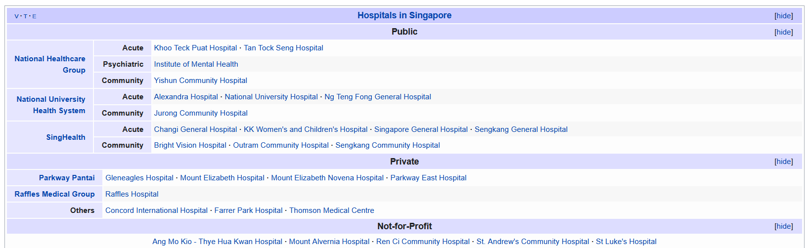
From there, I used Google and Healthhub to verify their postal codes.

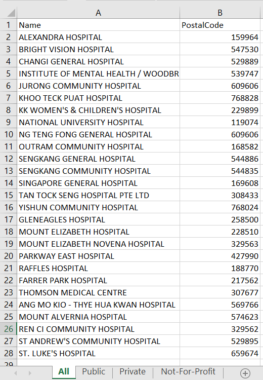
With this, we have our excel workbook! There’s an ‘All’ sheet which is the collation of all hospitals, and said hospitals are categorised under ‘Public’, ‘Private’ and ‘Not-for-Profit’ in their respective sheets. Our two columns are Name and PostalCode.
“But wait!” You might quip, “those are only postal codes. We need the longitude and latitude if we want to analyse this as geospatial data!”
No worries, dear reader! Our aim is to transform this .csv into a .shp, and that’s possible with our handy OneMapSG API - specifically, the search function. To use the search function, we have to specify:
searchVal: our search valuereturnGeom {Y/N}: whether we can to return the geometrygetAddrDetails {Y/N}: whether we want to return address details for a point
Let’s try using the postal code of Ren Ci Community Hospital (329562) as our search value!
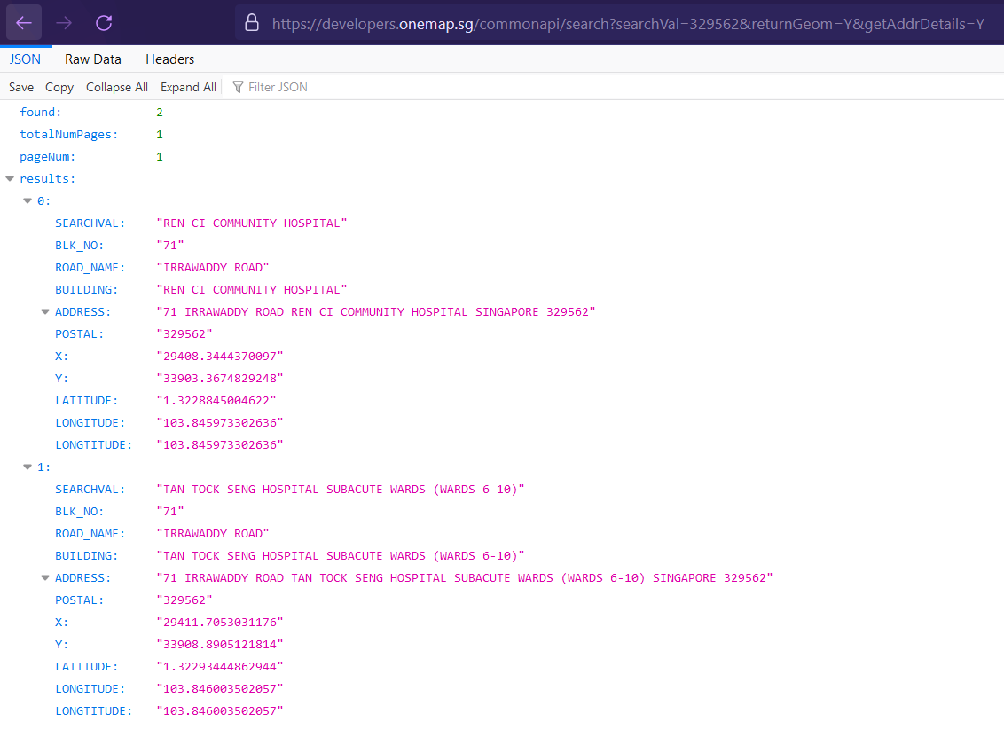
Oh no 😟 As we can see, there could be multiple results for a single postal code, and as we can see: each result has a slightly different longitude/latitude. To rectify this and narrow down to our desired result, we’ll add our hospital name to the search value:
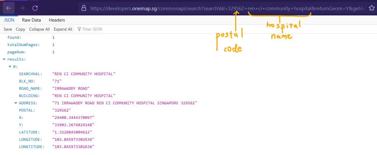
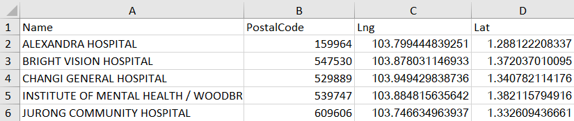
There we go! Afterwards, I collated the longitude and latitude and added it to the updated hospital excel file, hospitals_updated.xlsx, so it looks like this:
EDIT: in retrospect, I realised I could have tried pulling this data with GET requests (with the httr package) and parased the JSON (with the jsonlite package). Oh well - that’s something we can try in future works!
Note that some hospitals are integrated into a healthcare hub with a community hospital: in other words, they are near each other, or in the case of Jurong Community Hospital and Ng Teng Fong General Hospital, share the same postal code. As we’ve seen from our OneMapSG API that the same postal code has different latitude + longitude for different buildings, and knowing that they serve different purposes and different types of patients, I’ve opted to leave both types of hospitals in. However, you might want to take note of this for future work.
In addition, one of the hospitals listed on Wikipedia and Healthhub, “Concord International Hospital”, was reported to have suspended their healthcare services, but that article was followed up by a resumption of services, possibly under a new name.


In addition, Google has listed it as ‘permenanetly closed’.

Due to the uncertain conditions of Concord International Hospital, I’ve opted to leave it out of this dataset.
2.4 Good Primary Schools
Education and academic institutions are an especially important locational factors for families with children, or expect to have children. While some might be concerned about the number of schools around their house, I believe that most parents are focused only on the proxmimity to ‘good/elite schools’, especially when distance affects priority admission. For this analysis, our focus will be on the primary-school level of education - and only on the ‘good/elite’ schools. While MOE doesn’t release a ranking of the schools, we can roughly gauge the ‘rank’ from a number of factors:
- Popularity in Primary 1 (P1) Registration
- whether it offers the Gifted Education Programme (GEP)
- if there is a Special Assistance Plan (SAP)
- Achievements in the Singapore Youth Festival Arts Presentation
- Representation in the Singapore National School Games
- Singapore Uniformed Groups Unit Recognition
I’m referring to schlah’s Primary School Rankings, 2020 as they transparently state the weights given for each factor.
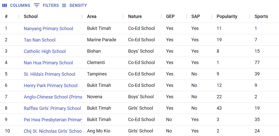
Like with the hospital dataset, I’ve made use of OneMapSG’s common api search function to find the longitude and latitudes of these primary schools and saved it in a new excel, top10_prisch_updated. Speaking of OneMapSG API… let’s look at how to use it in the next section!
2.5 Using the OneMapSG API
Last exercise, I met a wall with some authorisation issues with the OneMapSG API. But this time, I say goodbye to those worries - token in hand, I could make use of the API! I’d recommend reading its introductory document and its vignette to get a sensing as to how to use it. However, if you have similar authorisation issues, fret not: you can download the datasets from either data.gov.sg or LTA Data Mall. Check our this document for the list of available themes.
We’ve already discussed how to use the search function to help us with finding the longitude and latitude of our specified hospitals and primary schools - but what about whole datasets? Well, that’s possible, of course! In fact, we can even download them as shapefiles. Here’s my process for finding and downloading the relevant datasets:
- Before we start, be sure to have your token! I preloaded mine into a
tokenvariable for ease of access. - Search for the specified theme with
search_themes(token, "searchval")- for example, if I wanted to search for childcare services, I’d runsearch_themes(token, "childcare")in my console - [Optional] Check the theme status with
get_theme_status(token, "themename") - The theme dataset is a tibble dataframe, so we can retrieve and store it with
themetibble <- get_theme(token, "themename") - From here, we can convert our tibble dataframe to simple features dataframe. All the themes for this project use Lat and Lng as the latitude and longitude respectively, and our project coordinates system should be in the WGS84 system, aka ESPG code 4326. Thus,
themesf <- st_as_sf(themetibble, coords=c("Lng", "Lat"), crs=4326) - Now, we’ll need to write from an sf into a shapefile, which we can do with
st_write(themesf, "themename.shp")
Here’s the compilation of codes of the process, from start to finish:
Show code
# i used this set of codes and ran them in the console for each locational factor
# libraries should have been preloaded, but put here for reference of the necessary libraries!
library(sf)
library(onemapsgapi)
token <- "your value"
search_themes(token, "searchval")
get_theme_status(token, "themename")
themetibble <- get_theme(token, "themename")
themesf <- st_as_sf(themetibble, coords=c("Lng", "Lat"), crs=4326)
Things to look out for when using the API
Sometimes, when using search_themes to search for the datasets, your search value might turn up more than 10 results, but the tibble output auto-heads to the first 10 rows.
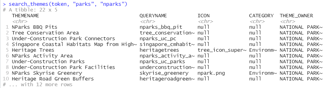
If you want to see more, what you can do is to add a %>%print(n=desiredval) after your code, like so:
Show code
# Reference: https://stackoverflow.com/questions/49122347/having-trouble-viewing-more-than-10-rows-in-a-tibble
search_themes(token, "parks", "nparks") %>% print(n = 25) #or your desired number
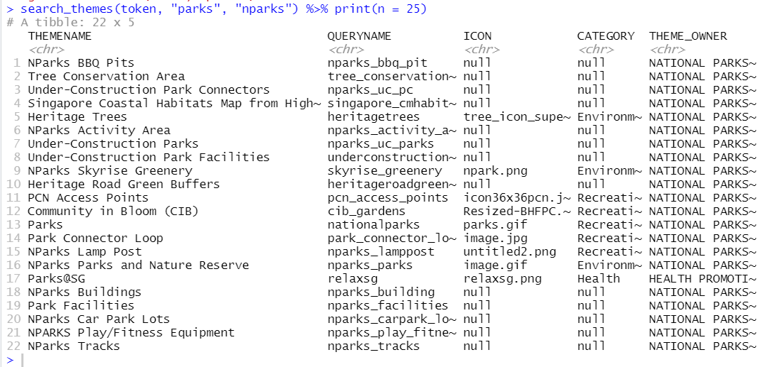
In addition, there might be similarly titles themes that both seem relevant to your analysis at first glance. For example, the same nparks query above has both “Parks” and “Nparks Parks and Nature Reserve”, uploaded by the National Parks Board. Which one should we pick? A closer look brings us to this:

Notice that “parks” is for recreational purposes, while “NParks Parks and Nature Reserve” were uploaded with environmental purposes in mind. Seeing as we’re trying to relate the locational factors to the pricing of resale housing units, it makes more sense to go with the former!
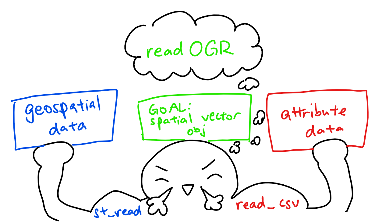
3.0 Data Wrangling: Geospatial Data
Here’s a lil refresher on the import methods:
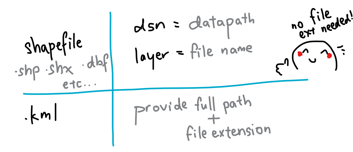
In addition, since we have .kml files - recall what we learned in our very first exercise, Hands-On Exercise 02:
3.1 Importing Geospatial Data
Base
Show code
# reads in geospatial data and stores into respective dataframes
sg_sf <- st_read(dsn = "data/geospatial", layer="CostalOutline")
Reading layer `CostalOutline' from data source
`C:\IS415\IS415_msty\_posts\2021-10-25-take-home-exercise-3\data\geospatial'
using driver `ESRI Shapefile'
Simple feature collection with 60 features and 4 fields
Geometry type: POLYGON
Dimension: XY
Bounding box: xmin: 2663.926 ymin: 16357.98 xmax: 56047.79 ymax: 50244.03
Projected CRS: SVY21Show code
mpsz_sf <- st_read(dsn = "data/geospatial", layer = "MP14_SUBZONE_WEB_PL")
Reading layer `MP14_SUBZONE_WEB_PL' from data source
`C:\IS415\IS415_msty\_posts\2021-10-25-take-home-exercise-3\data\geospatial'
using driver `ESRI Shapefile'
Simple feature collection with 323 features and 15 fields
Geometry type: MULTIPOLYGON
Dimension: XY
Bounding box: xmin: 2667.538 ymin: 15748.72 xmax: 56396.44 ymax: 50256.33
Projected CRS: SVY21Show code
rail_network_sf <- st_read(dsn="data/geospatial", layer="MRTLRTStnPtt")
Reading layer `MRTLRTStnPtt' from data source
`C:\IS415\IS415_msty\_posts\2021-10-25-take-home-exercise-3\data\geospatial'
using driver `ESRI Shapefile'
Simple feature collection with 171 features and 3 fields
Geometry type: POINT
Dimension: XY
Bounding box: xmin: 6138.311 ymin: 27555.06 xmax: 45254.86 ymax: 47854.2
Projected CRS: SVY21Show code
bus_sf <- st_read(dsn="data/geospatial", layer="BusStop")
Reading layer `BusStop' from data source
`C:\IS415\IS415_msty\_posts\2021-10-25-take-home-exercise-3\data\geospatial'
using driver `ESRI Shapefile'
Simple feature collection with 5156 features and 3 fields
Geometry type: POINT
Dimension: XY
Bounding box: xmin: 4427.938 ymin: 26482.1 xmax: 48282.5 ymax: 52983.82
Projected CRS: SVY21Extracted
Show code
childcare_sf <- st_read(dsn="data/geospatial/extracted", layer="childcare")
Reading layer `childcare' from data source
`C:\IS415\IS415_msty\_posts\2021-10-25-take-home-exercise-3\data\geospatial\extracted'
using driver `ESRI Shapefile'
Simple feature collection with 1545 features and 5 fields
Geometry type: POINT
Dimension: XY
Bounding box: xmin: 103.6824 ymin: 1.248403 xmax: 103.9897 ymax: 1.462134
Geodetic CRS: WGS 84Show code
eldercare_sf <- st_read(dsn="data/geospatial/extracted", layer="eldercare")
Reading layer `eldercare' from data source
`C:\IS415\IS415_msty\_posts\2021-10-25-take-home-exercise-3\data\geospatial\extracted'
using driver `ESRI Shapefile'
Simple feature collection with 133 features and 4 fields
Geometry type: POINT
Dimension: XY
Bounding box: xmin: 103.7119 ymin: 1.271472 xmax: 103.9561 ymax: 1.439561
Geodetic CRS: WGS 84Show code
hawkercentre_sf <- st_read(dsn="data/geospatial/extracted", layer="hawkercentres")
Reading layer `hawkercentres' from data source
`C:\IS415\IS415_msty\_posts\2021-10-25-take-home-exercise-3\data\geospatial\extracted'
using driver `ESRI Shapefile'
Simple feature collection with 125 features and 22 fields
Geometry type: POINT
Dimension: XY
Bounding box: xmin: 103.6974 ymin: 1.272716 xmax: 103.9882 ymax: 1.449217
Geodetic CRS: WGS 84Show code
kindergarten_sf <- st_read(dsn="data/geospatial/extracted", layer="kindergartens")
Reading layer `kindergartens' from data source
`C:\IS415\IS415_msty\_posts\2021-10-25-take-home-exercise-3\data\geospatial\extracted'
using driver `ESRI Shapefile'
Simple feature collection with 448 features and 5 fields
Geometry type: POINT
Dimension: XY
Bounding box: xmin: 103.6887 ymin: 1.247759 xmax: 103.9717 ymax: 1.455452
Geodetic CRS: WGS 84Show code
park_sf <- st_read(dsn="data/geospatial/extracted", layer="parks")
Reading layer `parks' from data source
`C:\IS415\IS415_msty\_posts\2021-10-25-take-home-exercise-3\data\geospatial\extracted'
using driver `ESRI Shapefile'
Simple feature collection with 352 features and 6 fields
Geometry type: POINT
Dimension: XY
Bounding box: xmin: 103.6929 ymin: 1.214058 xmax: 104.0017 ymax: 1.461503
Geodetic CRS: WGS 84Show code
supermarket_sf <- st_read(dsn="data/geospatial/extracted", layer="supermarkets")
Reading layer `supermarkets' from data source
`C:\IS415\IS415_msty\_posts\2021-10-25-take-home-exercise-3\data\geospatial\extracted'
using driver `ESRI Shapefile'
Simple feature collection with 526 features and 7 fields
Geometry type: POINT
Dimension: XY
Bounding box: xmin: 103.6258 ymin: 1.24715 xmax: 104.0036 ymax: 1.461526
Geodetic CRS: WGS 84Self-Sourced
Show code
chas_clinic_sf <- st_read("data/geospatial/selfsourced/chas-clinics-kml.kml")
Reading layer `MOH_CHAS_CLINICS' from data source
`C:\IS415\IS415_msty\_posts\2021-10-25-take-home-exercise-3\data\geospatial\selfsourced\chas-clinics-kml.kml'
using driver `KML'
Simple feature collection with 1167 features and 2 fields
Geometry type: POINT
Dimension: XYZ
Bounding box: xmin: 103.5818 ymin: 1.016264 xmax: 103.9903 ymax: 1.456037
z_range: zmin: 0 zmax: 0
Geodetic CRS: WGS 84Show code
isp_clinic_sf <- st_read(dsn="data/geospatial/selfsourced", layer="moh_isp_clinics")
Reading layer `moh_isp_clinics' from data source
`C:\IS415\IS415_msty\_posts\2021-10-25-take-home-exercise-3\data\geospatial\selfsourced'
using driver `ESRI Shapefile'
Simple feature collection with 378 features and 15 fields
Geometry type: POINT
Dimension: XY
Bounding box: xmin: 103.6907 ymin: 1.26397 xmax: 103.9903 ymax: 1.456037
Geodetic CRS: WGS 84Show code
malls <- read_csv("data/geospatial/selfsourced/mall_coordinates_updated.csv")
mall_sf <- st_as_sf(malls, coords = c("longitude", "latitude"), crs=4326)
hospitals <- read_excel("data/geospatial/selfsourced/hospitals_updated.xlsx")
hospitals_sf <-st_as_sf(hospitals, coords = c("Lng", "Lat"), crs=4326)
topprisch <- read_excel("data/geospatial/selfsourced/top10_prisch_updated.xlsx")
topprisch_sf <-st_as_sf(topprisch, coords = c("Lng", "Lat"), crs=4326)
As we can see, all of our ‘base’ datasets’ projected CRS is the ‘Singapore Projected Coordinate system’, SVY21 (ESPG Code 3414), which is appropriate for our Sinagpore-centric analysis. However, all the other datasets in ‘extracted’ and ‘selfsourced’ are using the ‘World Geodetic System 1984’, WGS84. We’ll address this and check on their CRS with st_crs() later on in Section 3.3.
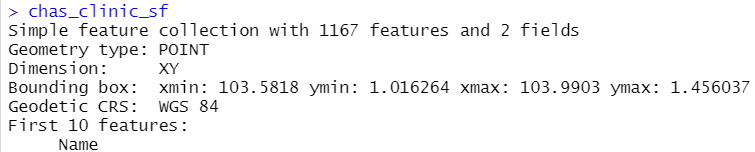
In addition, notice chas_clinic_sf has its dimensions listed as ‘XYZ’: it has a z-dimension, though as we can see from the z_range, both zmin and zmax are at 0. As it is irrelevant to our analysis, we’ll drop this with st_zm() in our pre-processing.
3.2 Data Pre-processing
Here are the things we need to check and tweak:
- Remove Z-Dimension (for chas_clinic_sf only)
- Removing unnecessary columns
- Check for invalid geometries
- Check for missing values
3.2.1 Removing Z-Dimensions
We’ll take care of the Z-Dimension of chas_clinic_sf with st_zm(), a function that drops Z (or M) dimensions from feature geometries and appropriately reset the classes.
Show code
# drops the Z-dimension from our dataframes
# due to the length of the output, I've opted to hide the results
chas_clinic_sf <- st_zm(chas_clinic_sf)
Show code
# once again, due to the length of output, I've opted to leave this as a non-evaluated line of code
# however, I've included a screenshot of the first portion of the output!
chas_clinic_sf
3.2.2 Removing Unnecessary Colummns
For most of our locational factor dataframes, the only thing we need to know is the name of the facility (childcare centre, eldercare etc.) and its geometry columm. As such, we only need to keep the first (name) column with select(c(1)) or select(1).
Show code
childcare_sf <- childcare_sf %>%
select(c(1))
eldercare_sf <- eldercare_sf %>%
select(c(1))
hawkercentre_sf <- hawkercentre_sf %>%
select(c(1))
kindergarten_sf <- kindergarten_sf %>%
select(c(1))
park_sf <- park_sf %>%
select(c(1))
supermarket_sf <- supermarket_sf %>%
select(c(1))
chas_clinic_sf <- chas_clinic_sf %>%
select(c(1))
isp_clinic_sf <- isp_clinic_sf %>%
select(c(1))
hospitals_sf <- hospitals_sf %>%
select(c(1))
topprisch_sf <- topprisch_sf %>%
select(c(1))
#for the mall_sf, the first column is actually the number, so we select the second column insteaed
mall_sf <- mall_sf %>%
select(c(2))
3.2.3 Invalid Geometries
Show code
# function breakdown:
# the st_is_valid function checks whether a geometry is valid
# which returns the indices of certain values based on logical conditions
# length returns the length of data objects
# checks for the number of geometries that are NOT valid
length(which(st_is_valid(sg_sf) == FALSE))
[1] 1Show code
length(which(st_is_valid(mpsz_sf) == FALSE))
[1] 9Show code
length(which(st_is_valid(rail_network_sf) == FALSE))
[1] 0Show code
length(which(st_is_valid(bus_sf) == FALSE))
[1] 0Show code
length(which(st_is_valid(childcare_sf) == FALSE))
[1] 0Show code
length(which(st_is_valid(eldercare_sf) == FALSE))
[1] 0Show code
length(which(st_is_valid(hawkercentre_sf) == FALSE))
[1] 0Show code
length(which(st_is_valid(kindergarten_sf) == FALSE))
[1] 0Show code
length(which(st_is_valid(park_sf) == FALSE))
[1] 0Show code
length(which(st_is_valid(supermarket_sf) == FALSE))
[1] 0Show code
length(which(st_is_valid(chas_clinic_sf) == FALSE))
[1] 0Show code
length(which(st_is_valid(isp_clinic_sf) == FALSE))
[1] 0Show code
length(which(st_is_valid(mall_sf) == FALSE))
[1] 0Show code
length(which(st_is_valid(hospitals_sf) == FALSE))
[1] 0Show code
length(which(st_is_valid(topprisch_sf) == FALSE))
[1] 0Show code
# Alternative Method
# test <- st_is_valid(sg_sf,reason=TRUE)
# length(which(test!= "Valid Geometry"))
# credit to Rajiv Abraham Xavier https://rpubs.com/rax/Take_Home_Ex01
As we can see from the output, sg has 1 invalid geometry while mpsz has 9 invalid geometries. With reference to this article on checking and creating validity, let’s address them and check again:
Show code
# st_make_valid takes in an invalid geometry and outputs a valid one with the lwgeom_makevalid method
sg_sf <- st_make_valid(sg_sf)
length(which(st_is_valid(sg_sf) == FALSE))
[1] 0Show code
mpsz_sf <- st_make_valid(mpsz_sf)
length(which(st_is_valid(mpsz_sf) == FALSE))
[1] 0Success! 🎉
3.2.4 Missing Values
Base
Show code
Simple feature collection with 0 features and 4 fields
Bounding box: xmin: NA ymin: NA xmax: NA ymax: NA
Projected CRS: SVY21
[1] GDO_GID MSLINK MAPID COSTAL_NAM geometry
<0 rows> (or 0-length row.names)Simple feature collection with 0 features and 15 fields
Bounding box: xmin: NA ymin: NA xmax: NA ymax: NA
Projected CRS: SVY21
[1] OBJECTID SUBZONE_NO SUBZONE_N SUBZONE_C CA_IND PLN_AREA_N
[7] PLN_AREA_C REGION_N REGION_C INC_CRC FMEL_UPD_D X_ADDR
[13] Y_ADDR SHAPE_Leng SHAPE_Area geometry
<0 rows> (or 0-length row.names)Simple feature collection with 0 features and 3 fields
Bounding box: xmin: NA ymin: NA xmax: NA ymax: NA
Projected CRS: SVY21
[1] OBJECTID STN_NAME STN_NO geometry
<0 rows> (or 0-length row.names)Simple feature collection with 1 feature and 3 fields
Geometry type: POINT
Dimension: XY
Bounding box: xmin: 22616.75 ymin: 47793.68 xmax: 22616.75 ymax: 47793.68
Projected CRS: SVY21
BUS_STOP_N BUS_ROOF_N LOC_DESC geometry
264 47201 UNK <NA> POINT (22616.75 47793.68)Extracted
Simple feature collection with 0 features and 1 field
Bounding box: xmin: NA ymin: NA xmax: NA ymax: NA
Geodetic CRS: WGS 84
[1] NAME geometry
<0 rows> (or 0-length row.names)Simple feature collection with 0 features and 1 field
Bounding box: xmin: NA ymin: NA xmax: NA ymax: NA
Geodetic CRS: WGS 84
[1] NAME geometry
<0 rows> (or 0-length row.names)Simple feature collection with 0 features and 1 field
Bounding box: xmin: NA ymin: NA xmax: NA ymax: NA
Geodetic CRS: WGS 84
[1] NAME geometry
<0 rows> (or 0-length row.names)Simple feature collection with 0 features and 1 field
Bounding box: xmin: NA ymin: NA xmax: NA ymax: NA
Geodetic CRS: WGS 84
[1] NAME geometry
<0 rows> (or 0-length row.names)Simple feature collection with 0 features and 1 field
Bounding box: xmin: NA ymin: NA xmax: NA ymax: NA
Geodetic CRS: WGS 84
[1] NAME geometry
<0 rows> (or 0-length row.names)Simple feature collection with 0 features and 1 field
Bounding box: xmin: NA ymin: NA xmax: NA ymax: NA
Geodetic CRS: WGS 84
[1] NAME geometry
<0 rows> (or 0-length row.names)Self-Sourced
Simple feature collection with 0 features and 1 field
Bounding box: xmin: NA ymin: NA xmax: NA ymax: NA
Geodetic CRS: WGS 84
[1] Name geometry
<0 rows> (or 0-length row.names)Simple feature collection with 0 features and 1 field
Bounding box: xmin: NA ymin: NA xmax: NA ymax: NA
Geodetic CRS: WGS 84
[1] NAME geometry
<0 rows> (or 0-length row.names)Simple feature collection with 0 features and 1 field
Bounding box: xmin: NA ymin: NA xmax: NA ymax: NA
Geodetic CRS: WGS 84
# A tibble: 0 x 2
# ... with 2 variables: name <chr>, geometry <GEOMETRY [°]>Simple feature collection with 0 features and 1 field
Bounding box: xmin: NA ymin: NA xmax: NA ymax: NA
Geodetic CRS: WGS 84
# A tibble: 0 x 2
# ... with 2 variables: Name <chr>, geometry <GEOMETRY [°]>Simple feature collection with 0 features and 1 field
Bounding box: xmin: NA ymin: NA xmax: NA ymax: NA
Geodetic CRS: WGS 84
# A tibble: 0 x 2
# ... with 2 variables: School <chr>, geometry <GEOMETRY [°]>There’s a missing value in our bus_sf dataset, so let’s remove the NA observation:
And let’s check for missing values one last time, just to be sure:
Show code
Simple feature collection with 0 features and 3 fields
Bounding box: xmin: NA ymin: NA xmax: NA ymax: NA
Projected CRS: SVY21
[1] BUS_STOP_N BUS_ROOF_N LOC_DESC geometry
<0 rows> (or 0-length row.names)Alright, our geospatial data pre-processing is done! 🥳
Note: if you didn’t remove the unnecssary columns, you likely would’ve gotten a lot of NA across various datasets e.g. “descriptions” that aren’t filled in, and also would have columns unneeded for analysis e.g. “icons”. That’s why we narrow down to our necessary columns this time round!
3.3 Verifying + Transforming Coordinate System
When we imported the data, we made a mental note to verify the projected CRS - and we’ll do that now!
Base
Show code
# using st_crs() function to check on the CRS and ESPG Codes
st_crs(sg_sf)
Coordinate Reference System:
User input: SVY21
wkt:
PROJCRS["SVY21",
BASEGEOGCRS["SVY21[WGS84]",
DATUM["World Geodetic System 1984",
ELLIPSOID["WGS 84",6378137,298.257223563,
LENGTHUNIT["metre",1]],
ID["EPSG",6326]],
PRIMEM["Greenwich",0,
ANGLEUNIT["Degree",0.0174532925199433]]],
CONVERSION["unnamed",
METHOD["Transverse Mercator",
ID["EPSG",9807]],
PARAMETER["Latitude of natural origin",1.36666666666667,
ANGLEUNIT["Degree",0.0174532925199433],
ID["EPSG",8801]],
PARAMETER["Longitude of natural origin",103.833333333333,
ANGLEUNIT["Degree",0.0174532925199433],
ID["EPSG",8802]],
PARAMETER["Scale factor at natural origin",1,
SCALEUNIT["unity",1],
ID["EPSG",8805]],
PARAMETER["False easting",28001.642,
LENGTHUNIT["metre",1],
ID["EPSG",8806]],
PARAMETER["False northing",38744.572,
LENGTHUNIT["metre",1],
ID["EPSG",8807]]],
CS[Cartesian,2],
AXIS["(E)",east,
ORDER[1],
LENGTHUNIT["metre",1,
ID["EPSG",9001]]],
AXIS["(N)",north,
ORDER[2],
LENGTHUNIT["metre",1,
ID["EPSG",9001]]]]Show code
st_crs(mpsz_sf)
Coordinate Reference System:
User input: SVY21
wkt:
PROJCRS["SVY21",
BASEGEOGCRS["SVY21[WGS84]",
DATUM["World Geodetic System 1984",
ELLIPSOID["WGS 84",6378137,298.257223563,
LENGTHUNIT["metre",1]],
ID["EPSG",6326]],
PRIMEM["Greenwich",0,
ANGLEUNIT["Degree",0.0174532925199433]]],
CONVERSION["unnamed",
METHOD["Transverse Mercator",
ID["EPSG",9807]],
PARAMETER["Latitude of natural origin",1.36666666666667,
ANGLEUNIT["Degree",0.0174532925199433],
ID["EPSG",8801]],
PARAMETER["Longitude of natural origin",103.833333333333,
ANGLEUNIT["Degree",0.0174532925199433],
ID["EPSG",8802]],
PARAMETER["Scale factor at natural origin",1,
SCALEUNIT["unity",1],
ID["EPSG",8805]],
PARAMETER["False easting",28001.642,
LENGTHUNIT["metre",1],
ID["EPSG",8806]],
PARAMETER["False northing",38744.572,
LENGTHUNIT["metre",1],
ID["EPSG",8807]]],
CS[Cartesian,2],
AXIS["(E)",east,
ORDER[1],
LENGTHUNIT["metre",1,
ID["EPSG",9001]]],
AXIS["(N)",north,
ORDER[2],
LENGTHUNIT["metre",1,
ID["EPSG",9001]]]]Show code
st_crs(rail_network_sf)
Coordinate Reference System:
User input: SVY21
wkt:
PROJCRS["SVY21",
BASEGEOGCRS["SVY21[WGS84]",
DATUM["World Geodetic System 1984",
ELLIPSOID["WGS 84",6378137,298.257223563,
LENGTHUNIT["metre",1]],
ID["EPSG",6326]],
PRIMEM["Greenwich",0,
ANGLEUNIT["Degree",0.0174532925199433]]],
CONVERSION["unnamed",
METHOD["Transverse Mercator",
ID["EPSG",9807]],
PARAMETER["Latitude of natural origin",1.36666666666667,
ANGLEUNIT["Degree",0.0174532925199433],
ID["EPSG",8801]],
PARAMETER["Longitude of natural origin",103.833333333333,
ANGLEUNIT["Degree",0.0174532925199433],
ID["EPSG",8802]],
PARAMETER["Scale factor at natural origin",1,
SCALEUNIT["unity",1],
ID["EPSG",8805]],
PARAMETER["False easting",28001.642,
LENGTHUNIT["metre",1],
ID["EPSG",8806]],
PARAMETER["False northing",38744.572,
LENGTHUNIT["metre",1],
ID["EPSG",8807]]],
CS[Cartesian,2],
AXIS["(E)",east,
ORDER[1],
LENGTHUNIT["metre",1,
ID["EPSG",9001]]],
AXIS["(N)",north,
ORDER[2],
LENGTHUNIT["metre",1,
ID["EPSG",9001]]]]Show code
st_crs(bus_sf)
Coordinate Reference System:
User input: SVY21
wkt:
PROJCRS["SVY21",
BASEGEOGCRS["WGS 84",
DATUM["World Geodetic System 1984",
ELLIPSOID["WGS 84",6378137,298.257223563,
LENGTHUNIT["metre",1]],
ID["EPSG",6326]],
PRIMEM["Greenwich",0,
ANGLEUNIT["Degree",0.0174532925199433]]],
CONVERSION["unnamed",
METHOD["Transverse Mercator",
ID["EPSG",9807]],
PARAMETER["Latitude of natural origin",1.36666666666667,
ANGLEUNIT["Degree",0.0174532925199433],
ID["EPSG",8801]],
PARAMETER["Longitude of natural origin",103.833333333333,
ANGLEUNIT["Degree",0.0174532925199433],
ID["EPSG",8802]],
PARAMETER["Scale factor at natural origin",1,
SCALEUNIT["unity",1],
ID["EPSG",8805]],
PARAMETER["False easting",28001.642,
LENGTHUNIT["metre",1],
ID["EPSG",8806]],
PARAMETER["False northing",38744.572,
LENGTHUNIT["metre",1],
ID["EPSG",8807]]],
CS[Cartesian,2],
AXIS["(E)",east,
ORDER[1],
LENGTHUNIT["metre",1,
ID["EPSG",9001]]],
AXIS["(N)",north,
ORDER[2],
LENGTHUNIT["metre",1,
ID["EPSG",9001]]]]Extracted
Show code
st_crs(childcare_sf)
Coordinate Reference System:
User input: WGS 84
wkt:
GEOGCRS["WGS 84",
DATUM["World Geodetic System 1984",
ELLIPSOID["WGS 84",6378137,298.257223563,
LENGTHUNIT["metre",1]]],
PRIMEM["Greenwich",0,
ANGLEUNIT["degree",0.0174532925199433]],
CS[ellipsoidal,2],
AXIS["latitude",north,
ORDER[1],
ANGLEUNIT["degree",0.0174532925199433]],
AXIS["longitude",east,
ORDER[2],
ANGLEUNIT["degree",0.0174532925199433]],
ID["EPSG",4326]]Show code
st_crs(eldercare_sf)
Coordinate Reference System:
User input: WGS 84
wkt:
GEOGCRS["WGS 84",
DATUM["World Geodetic System 1984",
ELLIPSOID["WGS 84",6378137,298.257223563,
LENGTHUNIT["metre",1]]],
PRIMEM["Greenwich",0,
ANGLEUNIT["degree",0.0174532925199433]],
CS[ellipsoidal,2],
AXIS["latitude",north,
ORDER[1],
ANGLEUNIT["degree",0.0174532925199433]],
AXIS["longitude",east,
ORDER[2],
ANGLEUNIT["degree",0.0174532925199433]],
ID["EPSG",4326]]Show code
st_crs(hawkercentre_sf)
Coordinate Reference System:
User input: WGS 84
wkt:
GEOGCRS["WGS 84",
DATUM["World Geodetic System 1984",
ELLIPSOID["WGS 84",6378137,298.257223563,
LENGTHUNIT["metre",1]]],
PRIMEM["Greenwich",0,
ANGLEUNIT["degree",0.0174532925199433]],
CS[ellipsoidal,2],
AXIS["latitude",north,
ORDER[1],
ANGLEUNIT["degree",0.0174532925199433]],
AXIS["longitude",east,
ORDER[2],
ANGLEUNIT["degree",0.0174532925199433]],
ID["EPSG",4326]]Show code
st_crs(kindergarten_sf)
Coordinate Reference System:
User input: WGS 84
wkt:
GEOGCRS["WGS 84",
DATUM["World Geodetic System 1984",
ELLIPSOID["WGS 84",6378137,298.257223563,
LENGTHUNIT["metre",1]]],
PRIMEM["Greenwich",0,
ANGLEUNIT["degree",0.0174532925199433]],
CS[ellipsoidal,2],
AXIS["latitude",north,
ORDER[1],
ANGLEUNIT["degree",0.0174532925199433]],
AXIS["longitude",east,
ORDER[2],
ANGLEUNIT["degree",0.0174532925199433]],
ID["EPSG",4326]]Show code
st_crs(park_sf)
Coordinate Reference System:
User input: WGS 84
wkt:
GEOGCRS["WGS 84",
DATUM["World Geodetic System 1984",
ELLIPSOID["WGS 84",6378137,298.257223563,
LENGTHUNIT["metre",1]]],
PRIMEM["Greenwich",0,
ANGLEUNIT["degree",0.0174532925199433]],
CS[ellipsoidal,2],
AXIS["latitude",north,
ORDER[1],
ANGLEUNIT["degree",0.0174532925199433]],
AXIS["longitude",east,
ORDER[2],
ANGLEUNIT["degree",0.0174532925199433]],
ID["EPSG",4326]]Show code
st_crs(supermarket_sf)
Coordinate Reference System:
User input: WGS 84
wkt:
GEOGCRS["WGS 84",
DATUM["World Geodetic System 1984",
ELLIPSOID["WGS 84",6378137,298.257223563,
LENGTHUNIT["metre",1]]],
PRIMEM["Greenwich",0,
ANGLEUNIT["degree",0.0174532925199433]],
CS[ellipsoidal,2],
AXIS["latitude",north,
ORDER[1],
ANGLEUNIT["degree",0.0174532925199433]],
AXIS["longitude",east,
ORDER[2],
ANGLEUNIT["degree",0.0174532925199433]],
ID["EPSG",4326]]Self-Sourced
Show code
st_crs(chas_clinic_sf)
Coordinate Reference System:
User input: WGS 84
wkt:
GEOGCRS["WGS 84",
DATUM["World Geodetic System 1984",
ELLIPSOID["WGS 84",6378137,298.257223563,
LENGTHUNIT["metre",1]]],
PRIMEM["Greenwich",0,
ANGLEUNIT["degree",0.0174532925199433]],
CS[ellipsoidal,2],
AXIS["geodetic latitude (Lat)",north,
ORDER[1],
ANGLEUNIT["degree",0.0174532925199433]],
AXIS["geodetic longitude (Lon)",east,
ORDER[2],
ANGLEUNIT["degree",0.0174532925199433]],
ID["EPSG",4326]]Show code
st_crs(isp_clinic_sf)
Coordinate Reference System:
User input: WGS 84
wkt:
GEOGCRS["WGS 84",
DATUM["World Geodetic System 1984",
ELLIPSOID["WGS 84",6378137,298.257223563,
LENGTHUNIT["metre",1]]],
PRIMEM["Greenwich",0,
ANGLEUNIT["degree",0.0174532925199433]],
CS[ellipsoidal,2],
AXIS["latitude",north,
ORDER[1],
ANGLEUNIT["degree",0.0174532925199433]],
AXIS["longitude",east,
ORDER[2],
ANGLEUNIT["degree",0.0174532925199433]],
ID["EPSG",4326]]Show code
st_crs(mall_sf)
Coordinate Reference System:
User input: EPSG:4326
wkt:
GEOGCRS["WGS 84",
DATUM["World Geodetic System 1984",
ELLIPSOID["WGS 84",6378137,298.257223563,
LENGTHUNIT["metre",1]]],
PRIMEM["Greenwich",0,
ANGLEUNIT["degree",0.0174532925199433]],
CS[ellipsoidal,2],
AXIS["geodetic latitude (Lat)",north,
ORDER[1],
ANGLEUNIT["degree",0.0174532925199433]],
AXIS["geodetic longitude (Lon)",east,
ORDER[2],
ANGLEUNIT["degree",0.0174532925199433]],
USAGE[
SCOPE["Horizontal component of 3D system."],
AREA["World."],
BBOX[-90,-180,90,180]],
ID["EPSG",4326]]Show code
st_crs(hospitals_sf)
Coordinate Reference System:
User input: EPSG:4326
wkt:
GEOGCRS["WGS 84",
DATUM["World Geodetic System 1984",
ELLIPSOID["WGS 84",6378137,298.257223563,
LENGTHUNIT["metre",1]]],
PRIMEM["Greenwich",0,
ANGLEUNIT["degree",0.0174532925199433]],
CS[ellipsoidal,2],
AXIS["geodetic latitude (Lat)",north,
ORDER[1],
ANGLEUNIT["degree",0.0174532925199433]],
AXIS["geodetic longitude (Lon)",east,
ORDER[2],
ANGLEUNIT["degree",0.0174532925199433]],
USAGE[
SCOPE["Horizontal component of 3D system."],
AREA["World."],
BBOX[-90,-180,90,180]],
ID["EPSG",4326]]Show code
st_crs(topprisch_sf)
Coordinate Reference System:
User input: EPSG:4326
wkt:
GEOGCRS["WGS 84",
DATUM["World Geodetic System 1984",
ELLIPSOID["WGS 84",6378137,298.257223563,
LENGTHUNIT["metre",1]]],
PRIMEM["Greenwich",0,
ANGLEUNIT["degree",0.0174532925199433]],
CS[ellipsoidal,2],
AXIS["geodetic latitude (Lat)",north,
ORDER[1],
ANGLEUNIT["degree",0.0174532925199433]],
AXIS["geodetic longitude (Lon)",east,
ORDER[2],
ANGLEUNIT["degree",0.0174532925199433]],
USAGE[
SCOPE["Horizontal component of 3D system."],
AREA["World."],
BBOX[-90,-180,90,180]],
ID["EPSG",4326]]Hmm. That’s not right - our projected CRS should be SVY21 (ESPG Code 3414), but for our given data, the current ESPG Codes are 9001. In addition, some of our self-sourced/extracted datasets are in WG84 (ESPG Code 4326) as well. Let’s assign the correct ESPG Codes:
Show code
# with st_set_crs(), we can assign the appropriate ESPG Code
sg_sf <- st_set_crs(sg_sf, 3414)
mpsz_sf <- st_set_crs(mpsz_sf, 3414)
rail_network_sf <- st_set_crs(rail_network_sf, 3414)
bus_sf <- st_set_crs(bus_sf, 3414)
# with st_transform(), we can change from one CRS to another
childcare_sf <- st_transform(childcare_sf, crs=3414)
eldercare_sf <- st_transform(eldercare_sf, crs=3414)
hawkercentre_sf <- st_transform(hawkercentre_sf, crs=3414)
kindergarten_sf <- st_transform(kindergarten_sf, crs=3414)
park_sf <- st_transform(park_sf, crs=3414)
supermarket_sf <- st_transform(supermarket_sf, crs=3414)
chas_clinic_sf <- st_transform(chas_clinic_sf, crs=3414)
isp_clinic_sf <- st_transform(isp_clinic_sf, crs=3414)
hospitals_sf <- st_transform(hospitals_sf, crs=3414)
topprisch_sf <- st_transform(topprisch_sf, crs=3414)
mall_sf <- st_transform(mall_sf, crs=3414)
And now, let’s check if the CRS has been properly assigned:
Base
Show code
# using st_crs() function to check on the CRS and ESPG Codes
st_crs(sg_sf)
Coordinate Reference System:
User input: EPSG:3414
wkt:
PROJCRS["SVY21 / Singapore TM",
BASEGEOGCRS["SVY21",
DATUM["SVY21",
ELLIPSOID["WGS 84",6378137,298.257223563,
LENGTHUNIT["metre",1]]],
PRIMEM["Greenwich",0,
ANGLEUNIT["degree",0.0174532925199433]],
ID["EPSG",4757]],
CONVERSION["Singapore Transverse Mercator",
METHOD["Transverse Mercator",
ID["EPSG",9807]],
PARAMETER["Latitude of natural origin",1.36666666666667,
ANGLEUNIT["degree",0.0174532925199433],
ID["EPSG",8801]],
PARAMETER["Longitude of natural origin",103.833333333333,
ANGLEUNIT["degree",0.0174532925199433],
ID["EPSG",8802]],
PARAMETER["Scale factor at natural origin",1,
SCALEUNIT["unity",1],
ID["EPSG",8805]],
PARAMETER["False easting",28001.642,
LENGTHUNIT["metre",1],
ID["EPSG",8806]],
PARAMETER["False northing",38744.572,
LENGTHUNIT["metre",1],
ID["EPSG",8807]]],
CS[Cartesian,2],
AXIS["northing (N)",north,
ORDER[1],
LENGTHUNIT["metre",1]],
AXIS["easting (E)",east,
ORDER[2],
LENGTHUNIT["metre",1]],
USAGE[
SCOPE["Cadastre, engineering survey, topographic mapping."],
AREA["Singapore - onshore and offshore."],
BBOX[1.13,103.59,1.47,104.07]],
ID["EPSG",3414]]Show code
st_crs(mpsz_sf)
Coordinate Reference System:
User input: EPSG:3414
wkt:
PROJCRS["SVY21 / Singapore TM",
BASEGEOGCRS["SVY21",
DATUM["SVY21",
ELLIPSOID["WGS 84",6378137,298.257223563,
LENGTHUNIT["metre",1]]],
PRIMEM["Greenwich",0,
ANGLEUNIT["degree",0.0174532925199433]],
ID["EPSG",4757]],
CONVERSION["Singapore Transverse Mercator",
METHOD["Transverse Mercator",
ID["EPSG",9807]],
PARAMETER["Latitude of natural origin",1.36666666666667,
ANGLEUNIT["degree",0.0174532925199433],
ID["EPSG",8801]],
PARAMETER["Longitude of natural origin",103.833333333333,
ANGLEUNIT["degree",0.0174532925199433],
ID["EPSG",8802]],
PARAMETER["Scale factor at natural origin",1,
SCALEUNIT["unity",1],
ID["EPSG",8805]],
PARAMETER["False easting",28001.642,
LENGTHUNIT["metre",1],
ID["EPSG",8806]],
PARAMETER["False northing",38744.572,
LENGTHUNIT["metre",1],
ID["EPSG",8807]]],
CS[Cartesian,2],
AXIS["northing (N)",north,
ORDER[1],
LENGTHUNIT["metre",1]],
AXIS["easting (E)",east,
ORDER[2],
LENGTHUNIT["metre",1]],
USAGE[
SCOPE["Cadastre, engineering survey, topographic mapping."],
AREA["Singapore - onshore and offshore."],
BBOX[1.13,103.59,1.47,104.07]],
ID["EPSG",3414]]Show code
st_crs(rail_network_sf)
Coordinate Reference System:
User input: EPSG:3414
wkt:
PROJCRS["SVY21 / Singapore TM",
BASEGEOGCRS["SVY21",
DATUM["SVY21",
ELLIPSOID["WGS 84",6378137,298.257223563,
LENGTHUNIT["metre",1]]],
PRIMEM["Greenwich",0,
ANGLEUNIT["degree",0.0174532925199433]],
ID["EPSG",4757]],
CONVERSION["Singapore Transverse Mercator",
METHOD["Transverse Mercator",
ID["EPSG",9807]],
PARAMETER["Latitude of natural origin",1.36666666666667,
ANGLEUNIT["degree",0.0174532925199433],
ID["EPSG",8801]],
PARAMETER["Longitude of natural origin",103.833333333333,
ANGLEUNIT["degree",0.0174532925199433],
ID["EPSG",8802]],
PARAMETER["Scale factor at natural origin",1,
SCALEUNIT["unity",1],
ID["EPSG",8805]],
PARAMETER["False easting",28001.642,
LENGTHUNIT["metre",1],
ID["EPSG",8806]],
PARAMETER["False northing",38744.572,
LENGTHUNIT["metre",1],
ID["EPSG",8807]]],
CS[Cartesian,2],
AXIS["northing (N)",north,
ORDER[1],
LENGTHUNIT["metre",1]],
AXIS["easting (E)",east,
ORDER[2],
LENGTHUNIT["metre",1]],
USAGE[
SCOPE["Cadastre, engineering survey, topographic mapping."],
AREA["Singapore - onshore and offshore."],
BBOX[1.13,103.59,1.47,104.07]],
ID["EPSG",3414]]Show code
st_crs(bus_sf)
Coordinate Reference System:
User input: EPSG:3414
wkt:
PROJCRS["SVY21 / Singapore TM",
BASEGEOGCRS["SVY21",
DATUM["SVY21",
ELLIPSOID["WGS 84",6378137,298.257223563,
LENGTHUNIT["metre",1]]],
PRIMEM["Greenwich",0,
ANGLEUNIT["degree",0.0174532925199433]],
ID["EPSG",4757]],
CONVERSION["Singapore Transverse Mercator",
METHOD["Transverse Mercator",
ID["EPSG",9807]],
PARAMETER["Latitude of natural origin",1.36666666666667,
ANGLEUNIT["degree",0.0174532925199433],
ID["EPSG",8801]],
PARAMETER["Longitude of natural origin",103.833333333333,
ANGLEUNIT["degree",0.0174532925199433],
ID["EPSG",8802]],
PARAMETER["Scale factor at natural origin",1,
SCALEUNIT["unity",1],
ID["EPSG",8805]],
PARAMETER["False easting",28001.642,
LENGTHUNIT["metre",1],
ID["EPSG",8806]],
PARAMETER["False northing",38744.572,
LENGTHUNIT["metre",1],
ID["EPSG",8807]]],
CS[Cartesian,2],
AXIS["northing (N)",north,
ORDER[1],
LENGTHUNIT["metre",1]],
AXIS["easting (E)",east,
ORDER[2],
LENGTHUNIT["metre",1]],
USAGE[
SCOPE["Cadastre, engineering survey, topographic mapping."],
AREA["Singapore - onshore and offshore."],
BBOX[1.13,103.59,1.47,104.07]],
ID["EPSG",3414]]Extracted
Show code
st_crs(childcare_sf)
Coordinate Reference System:
User input: EPSG:3414
wkt:
PROJCRS["SVY21 / Singapore TM",
BASEGEOGCRS["SVY21",
DATUM["SVY21",
ELLIPSOID["WGS 84",6378137,298.257223563,
LENGTHUNIT["metre",1]]],
PRIMEM["Greenwich",0,
ANGLEUNIT["degree",0.0174532925199433]],
ID["EPSG",4757]],
CONVERSION["Singapore Transverse Mercator",
METHOD["Transverse Mercator",
ID["EPSG",9807]],
PARAMETER["Latitude of natural origin",1.36666666666667,
ANGLEUNIT["degree",0.0174532925199433],
ID["EPSG",8801]],
PARAMETER["Longitude of natural origin",103.833333333333,
ANGLEUNIT["degree",0.0174532925199433],
ID["EPSG",8802]],
PARAMETER["Scale factor at natural origin",1,
SCALEUNIT["unity",1],
ID["EPSG",8805]],
PARAMETER["False easting",28001.642,
LENGTHUNIT["metre",1],
ID["EPSG",8806]],
PARAMETER["False northing",38744.572,
LENGTHUNIT["metre",1],
ID["EPSG",8807]]],
CS[Cartesian,2],
AXIS["northing (N)",north,
ORDER[1],
LENGTHUNIT["metre",1]],
AXIS["easting (E)",east,
ORDER[2],
LENGTHUNIT["metre",1]],
USAGE[
SCOPE["Cadastre, engineering survey, topographic mapping."],
AREA["Singapore - onshore and offshore."],
BBOX[1.13,103.59,1.47,104.07]],
ID["EPSG",3414]]Show code
st_crs(eldercare_sf)
Coordinate Reference System:
User input: EPSG:3414
wkt:
PROJCRS["SVY21 / Singapore TM",
BASEGEOGCRS["SVY21",
DATUM["SVY21",
ELLIPSOID["WGS 84",6378137,298.257223563,
LENGTHUNIT["metre",1]]],
PRIMEM["Greenwich",0,
ANGLEUNIT["degree",0.0174532925199433]],
ID["EPSG",4757]],
CONVERSION["Singapore Transverse Mercator",
METHOD["Transverse Mercator",
ID["EPSG",9807]],
PARAMETER["Latitude of natural origin",1.36666666666667,
ANGLEUNIT["degree",0.0174532925199433],
ID["EPSG",8801]],
PARAMETER["Longitude of natural origin",103.833333333333,
ANGLEUNIT["degree",0.0174532925199433],
ID["EPSG",8802]],
PARAMETER["Scale factor at natural origin",1,
SCALEUNIT["unity",1],
ID["EPSG",8805]],
PARAMETER["False easting",28001.642,
LENGTHUNIT["metre",1],
ID["EPSG",8806]],
PARAMETER["False northing",38744.572,
LENGTHUNIT["metre",1],
ID["EPSG",8807]]],
CS[Cartesian,2],
AXIS["northing (N)",north,
ORDER[1],
LENGTHUNIT["metre",1]],
AXIS["easting (E)",east,
ORDER[2],
LENGTHUNIT["metre",1]],
USAGE[
SCOPE["Cadastre, engineering survey, topographic mapping."],
AREA["Singapore - onshore and offshore."],
BBOX[1.13,103.59,1.47,104.07]],
ID["EPSG",3414]]Show code
st_crs(hawkercentre_sf)
Coordinate Reference System:
User input: EPSG:3414
wkt:
PROJCRS["SVY21 / Singapore TM",
BASEGEOGCRS["SVY21",
DATUM["SVY21",
ELLIPSOID["WGS 84",6378137,298.257223563,
LENGTHUNIT["metre",1]]],
PRIMEM["Greenwich",0,
ANGLEUNIT["degree",0.0174532925199433]],
ID["EPSG",4757]],
CONVERSION["Singapore Transverse Mercator",
METHOD["Transverse Mercator",
ID["EPSG",9807]],
PARAMETER["Latitude of natural origin",1.36666666666667,
ANGLEUNIT["degree",0.0174532925199433],
ID["EPSG",8801]],
PARAMETER["Longitude of natural origin",103.833333333333,
ANGLEUNIT["degree",0.0174532925199433],
ID["EPSG",8802]],
PARAMETER["Scale factor at natural origin",1,
SCALEUNIT["unity",1],
ID["EPSG",8805]],
PARAMETER["False easting",28001.642,
LENGTHUNIT["metre",1],
ID["EPSG",8806]],
PARAMETER["False northing",38744.572,
LENGTHUNIT["metre",1],
ID["EPSG",8807]]],
CS[Cartesian,2],
AXIS["northing (N)",north,
ORDER[1],
LENGTHUNIT["metre",1]],
AXIS["easting (E)",east,
ORDER[2],
LENGTHUNIT["metre",1]],
USAGE[
SCOPE["Cadastre, engineering survey, topographic mapping."],
AREA["Singapore - onshore and offshore."],
BBOX[1.13,103.59,1.47,104.07]],
ID["EPSG",3414]]Show code
st_crs(kindergarten_sf)
Coordinate Reference System:
User input: EPSG:3414
wkt:
PROJCRS["SVY21 / Singapore TM",
BASEGEOGCRS["SVY21",
DATUM["SVY21",
ELLIPSOID["WGS 84",6378137,298.257223563,
LENGTHUNIT["metre",1]]],
PRIMEM["Greenwich",0,
ANGLEUNIT["degree",0.0174532925199433]],
ID["EPSG",4757]],
CONVERSION["Singapore Transverse Mercator",
METHOD["Transverse Mercator",
ID["EPSG",9807]],
PARAMETER["Latitude of natural origin",1.36666666666667,
ANGLEUNIT["degree",0.0174532925199433],
ID["EPSG",8801]],
PARAMETER["Longitude of natural origin",103.833333333333,
ANGLEUNIT["degree",0.0174532925199433],
ID["EPSG",8802]],
PARAMETER["Scale factor at natural origin",1,
SCALEUNIT["unity",1],
ID["EPSG",8805]],
PARAMETER["False easting",28001.642,
LENGTHUNIT["metre",1],
ID["EPSG",8806]],
PARAMETER["False northing",38744.572,
LENGTHUNIT["metre",1],
ID["EPSG",8807]]],
CS[Cartesian,2],
AXIS["northing (N)",north,
ORDER[1],
LENGTHUNIT["metre",1]],
AXIS["easting (E)",east,
ORDER[2],
LENGTHUNIT["metre",1]],
USAGE[
SCOPE["Cadastre, engineering survey, topographic mapping."],
AREA["Singapore - onshore and offshore."],
BBOX[1.13,103.59,1.47,104.07]],
ID["EPSG",3414]]Show code
st_crs(park_sf)
Coordinate Reference System:
User input: EPSG:3414
wkt:
PROJCRS["SVY21 / Singapore TM",
BASEGEOGCRS["SVY21",
DATUM["SVY21",
ELLIPSOID["WGS 84",6378137,298.257223563,
LENGTHUNIT["metre",1]]],
PRIMEM["Greenwich",0,
ANGLEUNIT["degree",0.0174532925199433]],
ID["EPSG",4757]],
CONVERSION["Singapore Transverse Mercator",
METHOD["Transverse Mercator",
ID["EPSG",9807]],
PARAMETER["Latitude of natural origin",1.36666666666667,
ANGLEUNIT["degree",0.0174532925199433],
ID["EPSG",8801]],
PARAMETER["Longitude of natural origin",103.833333333333,
ANGLEUNIT["degree",0.0174532925199433],
ID["EPSG",8802]],
PARAMETER["Scale factor at natural origin",1,
SCALEUNIT["unity",1],
ID["EPSG",8805]],
PARAMETER["False easting",28001.642,
LENGTHUNIT["metre",1],
ID["EPSG",8806]],
PARAMETER["False northing",38744.572,
LENGTHUNIT["metre",1],
ID["EPSG",8807]]],
CS[Cartesian,2],
AXIS["northing (N)",north,
ORDER[1],
LENGTHUNIT["metre",1]],
AXIS["easting (E)",east,
ORDER[2],
LENGTHUNIT["metre",1]],
USAGE[
SCOPE["Cadastre, engineering survey, topographic mapping."],
AREA["Singapore - onshore and offshore."],
BBOX[1.13,103.59,1.47,104.07]],
ID["EPSG",3414]]Show code
st_crs(supermarket_sf)
Coordinate Reference System:
User input: EPSG:3414
wkt:
PROJCRS["SVY21 / Singapore TM",
BASEGEOGCRS["SVY21",
DATUM["SVY21",
ELLIPSOID["WGS 84",6378137,298.257223563,
LENGTHUNIT["metre",1]]],
PRIMEM["Greenwich",0,
ANGLEUNIT["degree",0.0174532925199433]],
ID["EPSG",4757]],
CONVERSION["Singapore Transverse Mercator",
METHOD["Transverse Mercator",
ID["EPSG",9807]],
PARAMETER["Latitude of natural origin",1.36666666666667,
ANGLEUNIT["degree",0.0174532925199433],
ID["EPSG",8801]],
PARAMETER["Longitude of natural origin",103.833333333333,
ANGLEUNIT["degree",0.0174532925199433],
ID["EPSG",8802]],
PARAMETER["Scale factor at natural origin",1,
SCALEUNIT["unity",1],
ID["EPSG",8805]],
PARAMETER["False easting",28001.642,
LENGTHUNIT["metre",1],
ID["EPSG",8806]],
PARAMETER["False northing",38744.572,
LENGTHUNIT["metre",1],
ID["EPSG",8807]]],
CS[Cartesian,2],
AXIS["northing (N)",north,
ORDER[1],
LENGTHUNIT["metre",1]],
AXIS["easting (E)",east,
ORDER[2],
LENGTHUNIT["metre",1]],
USAGE[
SCOPE["Cadastre, engineering survey, topographic mapping."],
AREA["Singapore - onshore and offshore."],
BBOX[1.13,103.59,1.47,104.07]],
ID["EPSG",3414]]Self-Sourced
Show code
st_crs(chas_clinic_sf)
Coordinate Reference System:
User input: EPSG:3414
wkt:
PROJCRS["SVY21 / Singapore TM",
BASEGEOGCRS["SVY21",
DATUM["SVY21",
ELLIPSOID["WGS 84",6378137,298.257223563,
LENGTHUNIT["metre",1]]],
PRIMEM["Greenwich",0,
ANGLEUNIT["degree",0.0174532925199433]],
ID["EPSG",4757]],
CONVERSION["Singapore Transverse Mercator",
METHOD["Transverse Mercator",
ID["EPSG",9807]],
PARAMETER["Latitude of natural origin",1.36666666666667,
ANGLEUNIT["degree",0.0174532925199433],
ID["EPSG",8801]],
PARAMETER["Longitude of natural origin",103.833333333333,
ANGLEUNIT["degree",0.0174532925199433],
ID["EPSG",8802]],
PARAMETER["Scale factor at natural origin",1,
SCALEUNIT["unity",1],
ID["EPSG",8805]],
PARAMETER["False easting",28001.642,
LENGTHUNIT["metre",1],
ID["EPSG",8806]],
PARAMETER["False northing",38744.572,
LENGTHUNIT["metre",1],
ID["EPSG",8807]]],
CS[Cartesian,2],
AXIS["northing (N)",north,
ORDER[1],
LENGTHUNIT["metre",1]],
AXIS["easting (E)",east,
ORDER[2],
LENGTHUNIT["metre",1]],
USAGE[
SCOPE["Cadastre, engineering survey, topographic mapping."],
AREA["Singapore - onshore and offshore."],
BBOX[1.13,103.59,1.47,104.07]],
ID["EPSG",3414]]Show code
st_crs(isp_clinic_sf)
Coordinate Reference System:
User input: EPSG:3414
wkt:
PROJCRS["SVY21 / Singapore TM",
BASEGEOGCRS["SVY21",
DATUM["SVY21",
ELLIPSOID["WGS 84",6378137,298.257223563,
LENGTHUNIT["metre",1]]],
PRIMEM["Greenwich",0,
ANGLEUNIT["degree",0.0174532925199433]],
ID["EPSG",4757]],
CONVERSION["Singapore Transverse Mercator",
METHOD["Transverse Mercator",
ID["EPSG",9807]],
PARAMETER["Latitude of natural origin",1.36666666666667,
ANGLEUNIT["degree",0.0174532925199433],
ID["EPSG",8801]],
PARAMETER["Longitude of natural origin",103.833333333333,
ANGLEUNIT["degree",0.0174532925199433],
ID["EPSG",8802]],
PARAMETER["Scale factor at natural origin",1,
SCALEUNIT["unity",1],
ID["EPSG",8805]],
PARAMETER["False easting",28001.642,
LENGTHUNIT["metre",1],
ID["EPSG",8806]],
PARAMETER["False northing",38744.572,
LENGTHUNIT["metre",1],
ID["EPSG",8807]]],
CS[Cartesian,2],
AXIS["northing (N)",north,
ORDER[1],
LENGTHUNIT["metre",1]],
AXIS["easting (E)",east,
ORDER[2],
LENGTHUNIT["metre",1]],
USAGE[
SCOPE["Cadastre, engineering survey, topographic mapping."],
AREA["Singapore - onshore and offshore."],
BBOX[1.13,103.59,1.47,104.07]],
ID["EPSG",3414]]Show code
st_crs(mall_sf)
Coordinate Reference System:
User input: EPSG:3414
wkt:
PROJCRS["SVY21 / Singapore TM",
BASEGEOGCRS["SVY21",
DATUM["SVY21",
ELLIPSOID["WGS 84",6378137,298.257223563,
LENGTHUNIT["metre",1]]],
PRIMEM["Greenwich",0,
ANGLEUNIT["degree",0.0174532925199433]],
ID["EPSG",4757]],
CONVERSION["Singapore Transverse Mercator",
METHOD["Transverse Mercator",
ID["EPSG",9807]],
PARAMETER["Latitude of natural origin",1.36666666666667,
ANGLEUNIT["degree",0.0174532925199433],
ID["EPSG",8801]],
PARAMETER["Longitude of natural origin",103.833333333333,
ANGLEUNIT["degree",0.0174532925199433],
ID["EPSG",8802]],
PARAMETER["Scale factor at natural origin",1,
SCALEUNIT["unity",1],
ID["EPSG",8805]],
PARAMETER["False easting",28001.642,
LENGTHUNIT["metre",1],
ID["EPSG",8806]],
PARAMETER["False northing",38744.572,
LENGTHUNIT["metre",1],
ID["EPSG",8807]]],
CS[Cartesian,2],
AXIS["northing (N)",north,
ORDER[1],
LENGTHUNIT["metre",1]],
AXIS["easting (E)",east,
ORDER[2],
LENGTHUNIT["metre",1]],
USAGE[
SCOPE["Cadastre, engineering survey, topographic mapping."],
AREA["Singapore - onshore and offshore."],
BBOX[1.13,103.59,1.47,104.07]],
ID["EPSG",3414]]Show code
st_crs(hospitals_sf)
Coordinate Reference System:
User input: EPSG:3414
wkt:
PROJCRS["SVY21 / Singapore TM",
BASEGEOGCRS["SVY21",
DATUM["SVY21",
ELLIPSOID["WGS 84",6378137,298.257223563,
LENGTHUNIT["metre",1]]],
PRIMEM["Greenwich",0,
ANGLEUNIT["degree",0.0174532925199433]],
ID["EPSG",4757]],
CONVERSION["Singapore Transverse Mercator",
METHOD["Transverse Mercator",
ID["EPSG",9807]],
PARAMETER["Latitude of natural origin",1.36666666666667,
ANGLEUNIT["degree",0.0174532925199433],
ID["EPSG",8801]],
PARAMETER["Longitude of natural origin",103.833333333333,
ANGLEUNIT["degree",0.0174532925199433],
ID["EPSG",8802]],
PARAMETER["Scale factor at natural origin",1,
SCALEUNIT["unity",1],
ID["EPSG",8805]],
PARAMETER["False easting",28001.642,
LENGTHUNIT["metre",1],
ID["EPSG",8806]],
PARAMETER["False northing",38744.572,
LENGTHUNIT["metre",1],
ID["EPSG",8807]]],
CS[Cartesian,2],
AXIS["northing (N)",north,
ORDER[1],
LENGTHUNIT["metre",1]],
AXIS["easting (E)",east,
ORDER[2],
LENGTHUNIT["metre",1]],
USAGE[
SCOPE["Cadastre, engineering survey, topographic mapping."],
AREA["Singapore - onshore and offshore."],
BBOX[1.13,103.59,1.47,104.07]],
ID["EPSG",3414]]Show code
st_crs(topprisch_sf)
Coordinate Reference System:
User input: EPSG:3414
wkt:
PROJCRS["SVY21 / Singapore TM",
BASEGEOGCRS["SVY21",
DATUM["SVY21",
ELLIPSOID["WGS 84",6378137,298.257223563,
LENGTHUNIT["metre",1]]],
PRIMEM["Greenwich",0,
ANGLEUNIT["degree",0.0174532925199433]],
ID["EPSG",4757]],
CONVERSION["Singapore Transverse Mercator",
METHOD["Transverse Mercator",
ID["EPSG",9807]],
PARAMETER["Latitude of natural origin",1.36666666666667,
ANGLEUNIT["degree",0.0174532925199433],
ID["EPSG",8801]],
PARAMETER["Longitude of natural origin",103.833333333333,
ANGLEUNIT["degree",0.0174532925199433],
ID["EPSG",8802]],
PARAMETER["Scale factor at natural origin",1,
SCALEUNIT["unity",1],
ID["EPSG",8805]],
PARAMETER["False easting",28001.642,
LENGTHUNIT["metre",1],
ID["EPSG",8806]],
PARAMETER["False northing",38744.572,
LENGTHUNIT["metre",1],
ID["EPSG",8807]]],
CS[Cartesian,2],
AXIS["northing (N)",north,
ORDER[1],
LENGTHUNIT["metre",1]],
AXIS["easting (E)",east,
ORDER[2],
LENGTHUNIT["metre",1]],
USAGE[
SCOPE["Cadastre, engineering survey, topographic mapping."],
AREA["Singapore - onshore and offshore."],
BBOX[1.13,103.59,1.47,104.07]],
ID["EPSG",3414]]Whew, that’s a long output - but as we can see, it’s all good! 💡
3.4 Initial Visualisation
Now that we’ve finished our standard pre-processing, let’s try visualising our data:
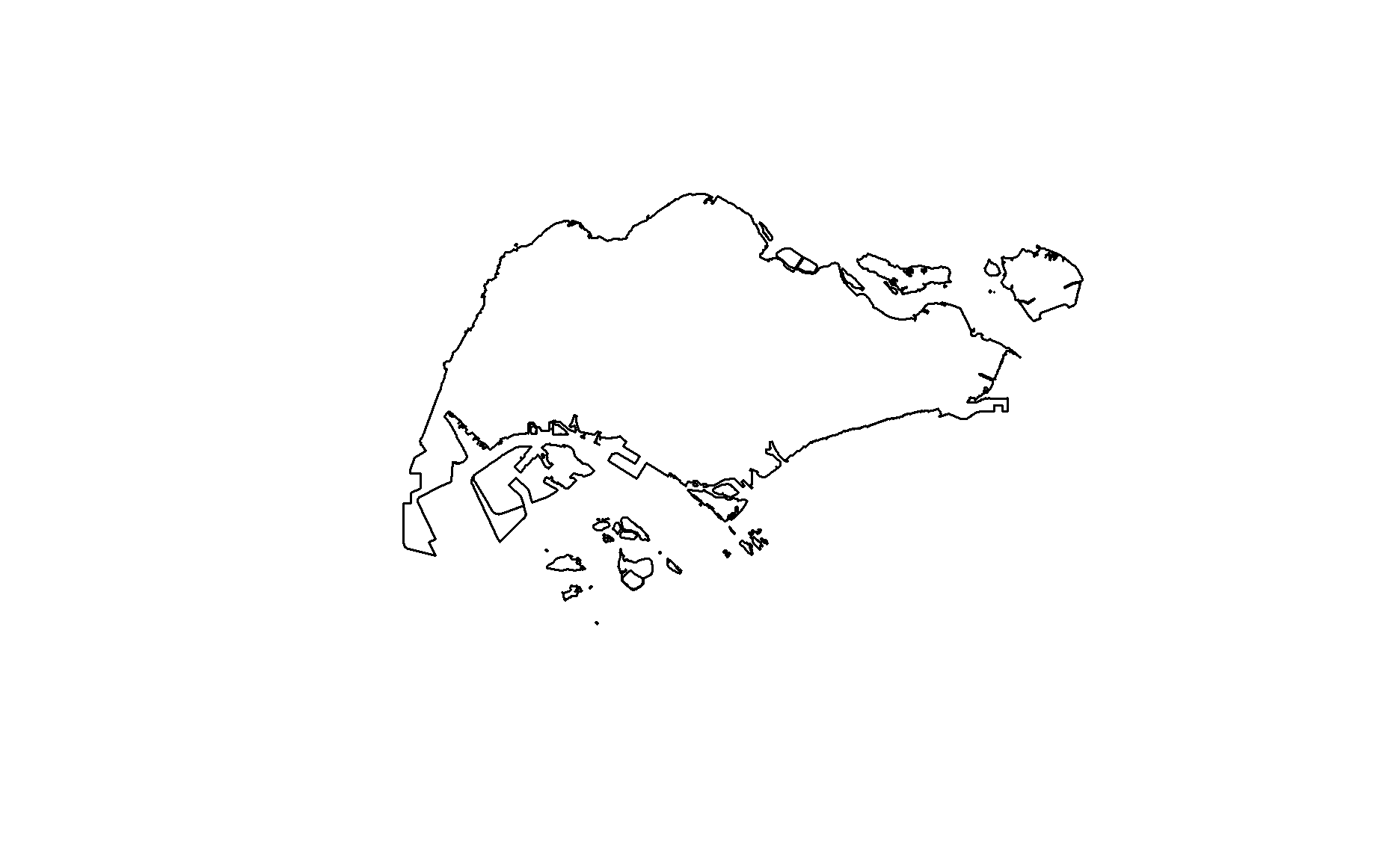
SG
Show code
# plots the geometry only - these are the 'base' maps
# alternatively, we can use plot(sg$geometry)
plot(st_geometry(sg_sf))
MPSZ
Show code
plot(st_geometry(mpsz_sf))
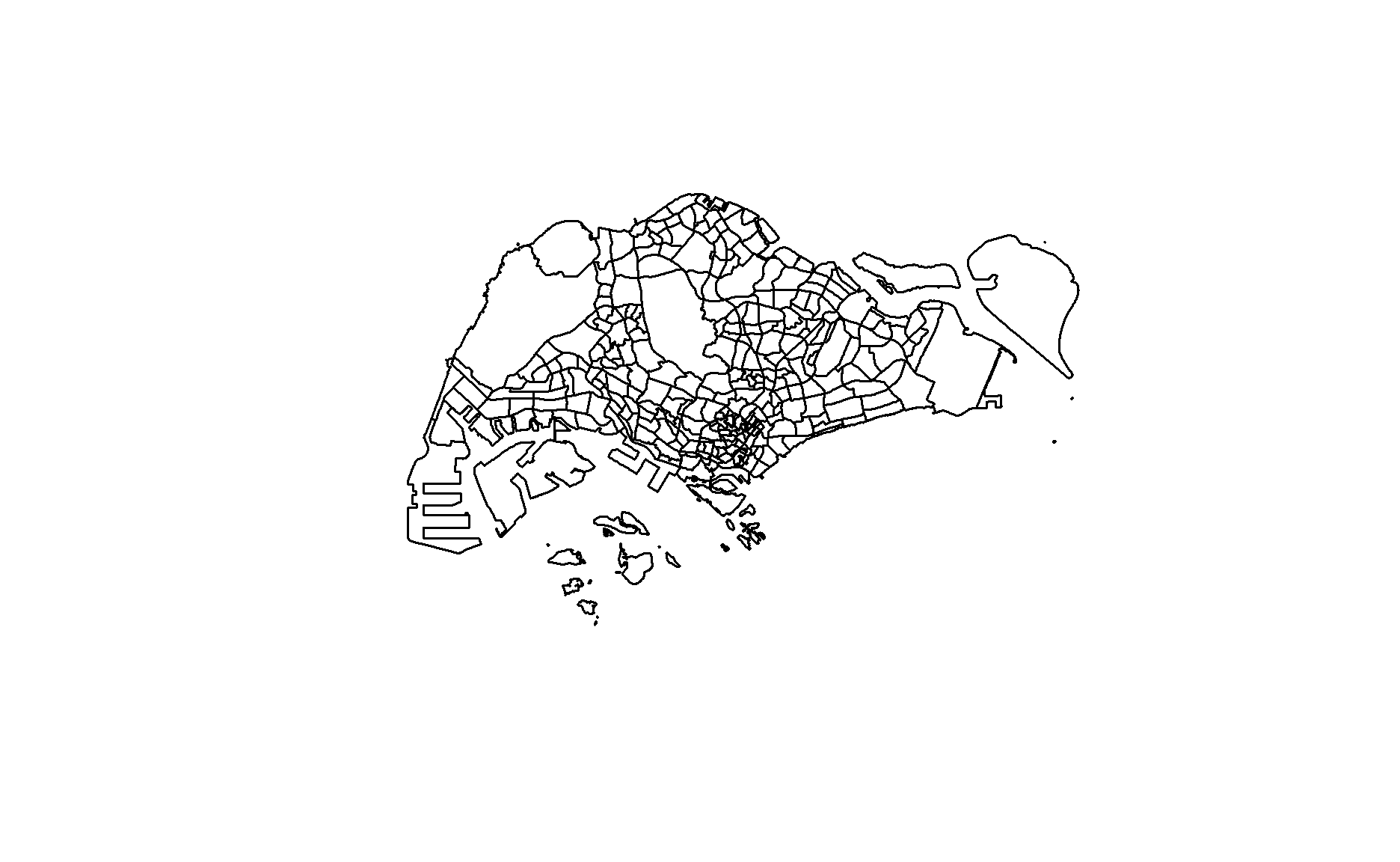
The main difference between sg and mpsz is that the former is a nationwide map, while the latter shows the subzones. Whichever we use depends on the scale of analysis: we might use sg for a general overview, while we’ll tap on the subzone divisions in mpsz if we want to look into specific subzones.
Show code
# switching to interactive map for better visualisation and to explore specific areas if needed
tmap_mode("view")
tm_shape(rail_network_sf) +
tm_dots(col="purple", size=0.05)
Show code
# return tmap mode to plot for future visualisations
tmap_mode("plot")
These are the MRT/LRT train stations. There are 3 distinct clusters - the two in the upper area, (West and Northeast regions specifically) are due to the LRT lines, while the cluster in the Central region is due interconnections of different lines in the CBD and city areas for increased connectivity
This also matches up to the existing railway network map:
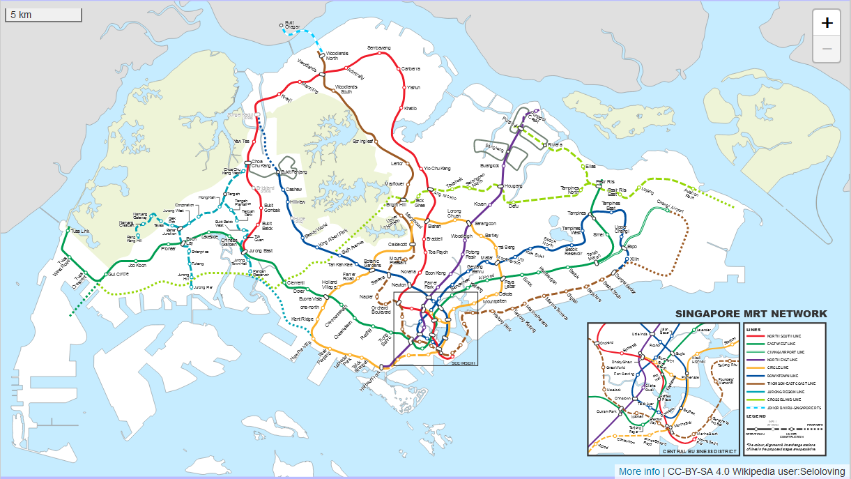
Retrieved from MRT.SG. Original work by Wikipedia user Seloloving.
Let’s also visualise the bus stops:
Show code
tmap_mode("plot")
tm_shape(mpsz_sf) +
tm_borders(alpha = 0.5) +
tmap_options(check.and.fix = TRUE) +
tm_shape(bus_sf) +
tm_dots(col="red", size=0.05) +
tm_layout(main.title = "Bus Stops",
main.title.position = "center",
main.title.size = 1.2,
frame = TRUE)
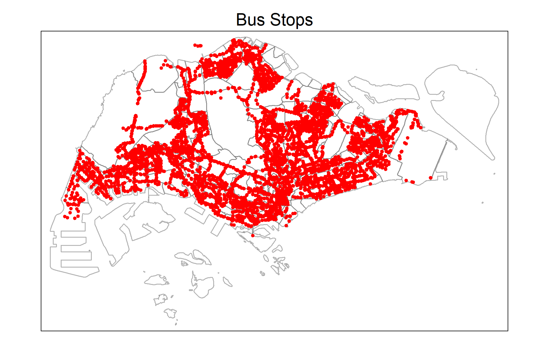
These is a good supplements to our railway_network - we can look at how the transport system and general connectivity of a place could play a role in determining the resale prices of housing units, especially since many citizens depend on the public transport system in their everyday lives due to its accessibility and cost.
Now, let’s view our other locations factors. Due to the amount of locational factors, I’ve opted to split them into the ‘recreational/lifestyle’ factors (hawker centres, parks, supermarkets, malls) and the ‘healthcare/education’ factors (childcare, eldercare, kindergartens, top primary schools, CHAS + ISP clinics, hospitals).
Recreational/Lifestyle
Show code
tmap_mode("view")
tm_shape(hawkercentre_sf) +
tm_dots(alpha=0.5, #affects transparency of points
col="#d62828",
size=0.05) +
tm_shape(park_sf) +
tm_dots(alpha=0.5,
col="#f77f00",
size=0.05) +
tm_shape(supermarket_sf) +
tm_dots(alpha=0.5,
col="#fcbf49",
size=0.05) +
tm_shape(mall_sf) +
tm_dots(alpha=0.5,
col="#eae2b7",
size=0.05)
Healthcare/Education
Show code
tmap_mode("view")
tm_shape(childcare_sf) +
tm_dots(alpha=0.5, #affects transparency of points
col="#2ec4b6",
size=0.05) +
tm_shape(eldercare_sf) +
tm_dots(alpha=0.5,
col="#e71d36",
size=0.05) +
tm_shape(kindergarten_sf) +
tm_dots(alpha=0.5,
col="#ff9f1c",
size=0.05) +
tm_shape(chas_clinic_sf) +
tm_dots(alpha=0.5,
col="#011627",
size=0.05) +
tm_shape(isp_clinic_sf) +
tm_dots(alpha=0.5,
col="#fdfffc",
size=0.05) +
tm_shape(hospitals_sf) +
tm_dots(alpha=0.5,
col="#6d597a",
size=0.05) +
tm_shape(topprisch_sf) +
tm_dots(alpha=0.5,
col="#f4acb7",
size=0.05)
4.0 Data Wrangling: Aspatial Data
4.1 Importing Aspatial Data
Now that we have our geospatial data sorted out, let’s move on to our aspatial data! We’ll need to import the data first. You might remember that in our last take-home exercise, we discovered the existence of duplicate columns when performing EDA. It’s important to understand what we’re working with and to check for any discrepancies! As such, after importing, let’s take a look at our dataframes with glimpse():
Import
Show code
# reads the the respective aspatial data and stores it as dataframes
# I've included show_col_types=FALSE so that there won't be a output of column types
# since in the next portion, we'll be using glimpse() to look at columns specifically
resale <- read_csv("data/aspatial/resale-flat-prices-based-on-registration-date-from-jan-2017-onwards.csv", show_col_types=FALSE)
Glimpse()
Show code
# gives an associated attribute information of the dataframe
glimpse(resale)
Rows: 111,633
Columns: 11
$ month <chr> "2017-01", "2017-01", "2017-01", "2017-0~
$ town <chr> "ANG MO KIO", "ANG MO KIO", "ANG MO KIO"~
$ flat_type <chr> "2 ROOM", "3 ROOM", "3 ROOM", "3 ROOM", ~
$ block <chr> "406", "108", "602", "465", "601", "150"~
$ street_name <chr> "ANG MO KIO AVE 10", "ANG MO KIO AVE 4",~
$ storey_range <chr> "10 TO 12", "01 TO 03", "01 TO 03", "04 ~
$ floor_area_sqm <dbl> 44, 67, 67, 68, 67, 68, 68, 67, 68, 67, ~
$ flat_model <chr> "Improved", "New Generation", "New Gener~
$ lease_commence_date <dbl> 1979, 1978, 1980, 1980, 1980, 1981, 1979~
$ remaining_lease <chr> "61 years 04 months", "60 years 07 month~
$ resale_price <dbl> 232000, 250000, 262000, 265000, 265000, ~Wait a moment… there’s no longitude and latitude features! In addition, keep in mind that we’re looking at four-room flat and a transaction period between 1st January 2019 to 30th September 2020.
Let’s filter the data, first:
Now, let’s geocode our aspatial data and add its longitude and latitude features with our OneMapSG API!
4.2 Geocoding our aspatial data
From my past experience with the search function of the OneMapSG API, I’ve realised that “ST.” is usually written as “SAINT” instead - for example, St. Luke’s Primary School is written as Saint Luke’s Primary School. To address, this, we’ll replace such occurrences:
Show code
resale$street_name <- gsub("ST\\.", "SAINT", resale$street_name)
Now, we let’s create the geocoding function! Here’s what we need to do:
- Combine the block and street name into an address
- Pass the address as the searchVal in our query
- Send the query to OneMapSG search Note: Since we don’t need all the address details, we can set
getAddrDetailsas ‘N’ - Convert response (JSON object) to text
- Save response in text form as a dataframe
- We only need to retain the latitude and longitude for our output
Show code
library(httr)
geocode <- function(block, streetname) {
base_url <- "https://developers.onemap.sg/commonapi/search"
address <- paste(block, streetname, sep = " ")
query <- list("searchVal" = address,
"returnGeom" = "Y",
"getAddrDetails" = "N",
"pageNum" = "1")
res <- GET(base_url, query = query)
restext<-content(res, as="text")
output <- fromJSON(restext) %>%
as.data.frame %>%
select(results.LATITUDE, results.LONGITUDE)
return(output)
}
Now, all we have to do is to execute the geocoding function:
Show code
resale$LATITUDE <- 0
resale$LONGITUDE <- 0
for (i in 1:nrow(resale)){
temp_output <- geocode(resale[i, 4], resale[i, 5])
resale$LATITUDE[i] <- temp_output$results.LATITUDE
resale$LONGITUDE[i] <- temp_output$results.LONGITUDE
}
4.3 Structural Factors
4.3.1 Floor Level
We need to conduct dummy coding on the storey_range variable if we want to use it in the model - but let’s first take a look at the storey_range values to get a rough idea:
Show code
unique(resale$storey_range)
[1] "10 TO 12" "01 TO 03" "04 TO 06" "07 TO 09" "13 TO 15" "19 TO 21"
[7] "22 TO 24" "16 TO 18" "34 TO 36" "28 TO 30" "37 TO 39" "49 TO 51"
[13] "25 TO 27" "40 TO 42" "31 TO 33" "46 TO 48" "43 TO 45"As we can see, there are 17 storey range categories. We’l use pivot_wider() and create duplicate variables representing every storey range, with the value being 1 if the observation belongs in said storey range, and 0 if otherwise.
4.3.1 Remaining Lease
Currently, the remaining_lease is in
Show code
str_list <- str_split(resale$remaining_lease, " ")
for (i in 1:length(str_list)) {
if (length(unlist(str_list[i])) > 2) {
year <- as.numeric(unlist(str_list[i])[1])
month <- as.numeric(unlist(str_list[i])[3])
resale$remaining_lease[i] <- year + round(month/12, 2)
}
else {
year <- as.numeric(unlist(str_list[i])[1])
resale$remaining_lease[i] <- year
}
}
4.4 Locational Factors - CBD
Lastly, we need to factor in the proximity to the Central Business District - in the Downtown Core. It’s located in the southwest of Singapore. As such, let’s take the coordinates of Downtown Core to be the coordinates of the CBD:
Show code
lat <- 1.287953
lng <- 103.851784
cbd_sf <- data.frame(lat, lng) %>%
st_as_sf(coords = c("lng", "lat"), crs=4326) %>%
st_transform(crs=3414)
4.5 Remaining Data Pre-Processing
4.5.1 Missing Values
Like with our geospatial data, we should check if there are missing values. We’re only concerned about the longitude and latitude specifically:
Note: PSST! If you’d like a way to show the number of NA values for columns with NA values only, I’d recommend checking this out.
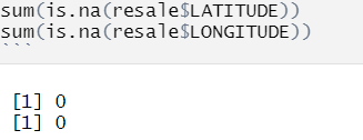
No NA values - we can move on!
4.5.2 Convert into sf objects + Transforming Coordinate System
Now, we have to transform our dataframe into an sf object, and then verify and transform our assigned CRS for our aspatial datasets. In fact, we already know that (just like some of our geospatial datasets above) resale uses WGS84 (ESPG Code 4326) on account of using Latitude and Longitude - so we can do these two things in one go:
Show code
# st_as_sf outputs a simple features data frame
resale_sf <- st_as_sf(resale,
coords = c("LONGITUDE",
"LATITUDE"),
# the geographical features are in longitude & latitude, in decimals
# as such, WGS84 is the most appropriate coordinates system
crs=4326) %>%
#afterwards, we transform it to SVY21, our desired CRS
st_transform(crs = 3414)
4.6 Proximity Distance Calculation
One of the things we need to find is the proximity to particular facilities - which we can compute with st_distance(), and find the closest facility (shortest distance) with the rowMins() function of our matrixStats package. The values will be appended to the data frame as a new column.
Show code
proximity <- function(df1, df2, varname) {
dist_matrix <- st_distance(df1, df2) %>%
drop_units()
df1[,varname] <- rowMins(dist_matrix)
return(df1)
}
Let’s implement it!
Show code
resale_sf <-
# the columns will be truncated later on when viewing
# so we're limiting ourselves to two-character columns for ease of viewing between
proximity(resale_sf, cbd_sf, "PROX_CBD") %>%
proximity(., childcare_sf, "PROX_CHILDCARE") %>%
proximity(., eldercare_sf, "PROX_ELDERCARE") %>%
proximity(., hawkercentre_sf, "PROX_HAWKER") %>%
proximity(., rail_network_sf, "PROX_MRT") %>%
proximity(., park_sf, "PROX_PARK") %>%
proximity(., topprisch_sf, "PROX_TOPPRISCH") %>%
proximity(., mall_sf, "PROX_MALL") %>%
proximity(., supermarket_sf, "PROX_SPRMKT") %>%
proximity(., hospitals_sf, "PROX_HOSPITAL")
4.7 Facility Count within Radius Calculation
Other than proxmity, which calculates the shortest distance, we also want to find the number of facilities within a particular radius. Like above, we’ll use st_distance() to compute the distance between the flats and the desried facilities, and then sum up the observations with rowSums(). The values will be appended to the data frame as a new column.
Show code
num_radius <- function(df1, df2, varname, radius) {
dist_matrix <- st_distance(df1, df2) %>%
drop_units() %>%
as.data.frame()
df1[,varname] <- rowSums(dist_matrix <= radius)
return(df1)
}
Now, let’s implement it!
4.8 Saving the Dataset
Phew! That took a long time to load… I’d rather not have to rerun all those pre-processing fucntiosna gain, so let’s this dataframe as a shapefile and read it in when we need it!
Before saving the dataset, let’s rename the columns to shorter forms and relocate the price column to the front of the data frame, like so:
Show code
resale_sf <- resale_sf %>%
# sometimes, you might get an internal error: can't find `agr` columns
# to circumvent, have an empty mutate()
# you won't affect your columns, but it corrects the agr attribute names
# reference: https://github.com/r-spatial/sf/issues/1472
mutate() %>%
rename("AREA_SQM" = "floor_area_sqm",
"LEASE_YRS" = "remaining_lease",
"PRICE"= "resale_price") %>%
relocate(`PRICE`)
We can now save the final flat resale price data set as a SHP file using st_write of sf package.
Show code
st_write(resale_sf, "data/geospatial/resale-final.shp")
5.0 Exploratory Data Analysis
Now, we can finally move on into EDA! Let’s start by loading and taking a look at our dataset:
Show code
resale_sf <- st_read(dsn="data/geospatial", layer="resale-final")
Reading layer `resale-final' from data source
`C:\IS415\IS415_msty\_posts\2021-10-25-take-home-exercise-3\data\geospatial'
using driver `ESRI Shapefile'
Simple feature collection with 15853 features and 42 fields
Geometry type: POINT
Dimension: XY
Bounding box: xmin: 11597.31 ymin: 28217.39 xmax: 42623.63 ymax: 48741.06
Projected CRS: SVY21 / Singapore TMShow code
glimpse(resale_sf)
Rows: 15,853
Columns: 43
$ PRICE <dbl> 330000, 360000, 370000, 375000, 380000, 380000, 385~
$ month <chr> "2019-01", "2019-01", "2019-01", "2019-01", "2019-0~
$ town <chr> "ANG MO KIO", "ANG MO KIO", "ANG MO KIO", "ANG MO K~
$ flt_typ <chr> "4 ROOM", "4 ROOM", "4 ROOM", "4 ROOM", "4 ROOM", "~
$ block <chr> "204", "175", "543", "118", "411", "546", "428", "1~
$ strt_nm <chr> "ANG MO KIO AVE 3", "ANG MO KIO AVE 4", "ANG MO KIO~
$ AREA_SQ <dbl> 92, 91, 92, 99, 92, 92, 92, 92, 93, 91, 91, 98, 92,~
$ flt_mdl <chr> "New Generation", "New Generation", "New Generation~
$ ls_cmm_ <dbl> 1977, 1981, 1981, 1978, 1979, 1981, 1978, 1982, 198~
$ LEASE_Y <chr> "57", "61.5", "61.08", "58.33", "59.58", "61", "58.~
$ X01TO03 <dbl> 1, 0, 1, 0, 0, 0, 0, 0, 0, 0, 0, 0, 0, 0, 0, 0, 0, ~
$ X07TO09 <dbl> 0, 1, 0, 0, 0, 0, 1, 0, 0, 1, 1, 1, 0, 1, 0, 0, 0, ~
$ X04TO06 <dbl> 0, 0, 0, 1, 1, 0, 0, 1, 0, 0, 0, 0, 0, 0, 1, 0, 0, ~
$ X10TO12 <dbl> 0, 0, 0, 0, 0, 1, 0, 0, 1, 0, 0, 0, 1, 0, 0, 0, 0, ~
$ X13TO15 <dbl> 0, 0, 0, 0, 0, 0, 0, 0, 0, 0, 0, 0, 0, 0, 0, 1, 1, ~
$ X25TO27 <dbl> 0, 0, 0, 0, 0, 0, 0, 0, 0, 0, 0, 0, 0, 0, 0, 0, 0, ~
$ X19TO21 <dbl> 0, 0, 0, 0, 0, 0, 0, 0, 0, 0, 0, 0, 0, 0, 0, 0, 0, ~
$ X16TO18 <dbl> 0, 0, 0, 0, 0, 0, 0, 0, 0, 0, 0, 0, 0, 0, 0, 0, 0, ~
$ X28TO30 <dbl> 0, 0, 0, 0, 0, 0, 0, 0, 0, 0, 0, 0, 0, 0, 0, 0, 0, ~
$ X31TO33 <dbl> 0, 0, 0, 0, 0, 0, 0, 0, 0, 0, 0, 0, 0, 0, 0, 0, 0, ~
$ X22TO24 <dbl> 0, 0, 0, 0, 0, 0, 0, 0, 0, 0, 0, 0, 0, 0, 0, 0, 0, ~
$ X37TO39 <dbl> 0, 0, 0, 0, 0, 0, 0, 0, 0, 0, 0, 0, 0, 0, 0, 0, 0, ~
$ X34TO36 <dbl> 0, 0, 0, 0, 0, 0, 0, 0, 0, 0, 0, 0, 0, 0, 0, 0, 0, ~
$ X40TO42 <dbl> 0, 0, 0, 0, 0, 0, 0, 0, 0, 0, 0, 0, 0, 0, 0, 0, 0, ~
$ X43TO45 <dbl> 0, 0, 0, 0, 0, 0, 0, 0, 0, 0, 0, 0, 0, 0, 0, 0, 0, ~
$ X46TO48 <dbl> 0, 0, 0, 0, 0, 0, 0, 0, 0, 0, 0, 0, 0, 0, 0, 0, 0, ~
$ X49TO51 <dbl> 0, 0, 0, 0, 0, 0, 0, 0, 0, 0, 0, 0, 0, 0, 0, 0, 0, ~
$ PROX_CB <dbl> 8824.749, 9841.309, 9560.780, 9609.731, 8351.051, 9~
$ PROX_CH <dbl> 1.909015e+02, 1.354044e+02, 8.016387e+01, 1.896699e~
$ PROX_EL <dbl> 251.4065, 631.8448, 1082.4168, 347.3195, 195.8226, ~
$ PROX_HA <dbl> 441.82653, 269.72560, 258.29513, 436.47518, 70.0908~
$ PROX_MR <dbl> 703.9715, 403.4297, 889.9529, 200.9786, 886.7502, 9~
$ PROX_PA <dbl> 745.0859, 429.4870, 780.0777, 177.6163, 913.3875, 8~
$ PROX_TO <dbl> 1270.3931, 404.5792, 2448.0584, 137.5070, 1502.8928~
$ PROX_MA <dbl> 546.0425, 1452.7315, 1030.7966, 1514.3828, 994.3982~
$ PROX_SP <dbl> 270.8222, 310.1889, 318.7560, 458.6748, 337.9803, 3~
$ PROX_HO <dbl> 1884.9254, 986.8126, 2068.9364, 1305.5690, 2706.972~
$ NUM_KND <dbl> 1, 1, 1, 1, 1, 1, 1, 1, 1, 0, 1, 1, 1, 1, 1, 2, 2, ~
$ NUM_CHI <dbl> 6, 5, 2, 3, 3, 2, 3, 4, 3, 2, 4, 4, 4, 5, 2, 7, 8, ~
$ NUM_BUS <dbl> 8, 8, 8, 7, 6, 9, 6, 6, 5, 4, 10, 5, 6, 9, 8, 4, 6,~
$ NUM_ISP <dbl> 0, 3, 1, 2, 2, 1, 3, 1, 2, 0, 3, 0, 3, 2, 2, 4, 3, ~
$ NUM_CHA <dbl> 2, 6, 6, 2, 5, 5, 7, 1, 7, 2, 4, 2, 7, 7, 4, 6, 6, ~
$ geometry <POINT [m]> POINT (29179.92 38822.08), POINT (28423.42 39~Notice that LEASE_YRS is still in string format - we’ve got to update that to a numeric format:
Show code
# had to use the truncated version!
resale_sf$LEASE_Y <- as.numeric(resale_sf$LEASE_Y)
Show code
summary(resale_sf$PRICE)
Min. 1st Qu. Median Mean 3rd Qu. Max.
218000 352800 405000 433563 470000 1186888 5.1 Statistical Graphics
We can start by plotting the distribution of selling price:
Show code
ggplot(data=resale_sf, aes(x=`PRICE`)) +
geom_histogram(bins=20, color="black", fill="light blue") +
labs(title = "Distribution of Resale Prices",
x = "Resale Prices",
y = 'Frequency')
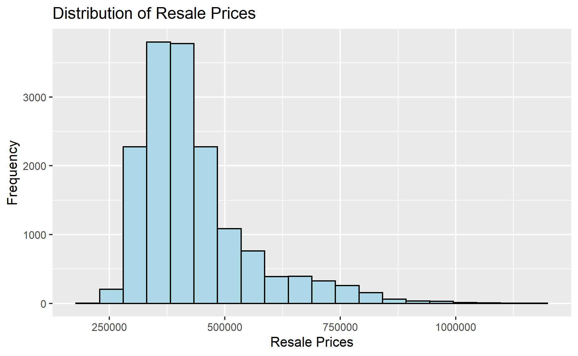
The figure above reveals a right skewed distribution. This means that more 4-room housing units were transacted at relative lower prices.
Statistically, the skewed distribution can be normalised by using log transformation - which we’ll derive with the mutate() function of the dplyr package and store in a new variable, like so:
Show code
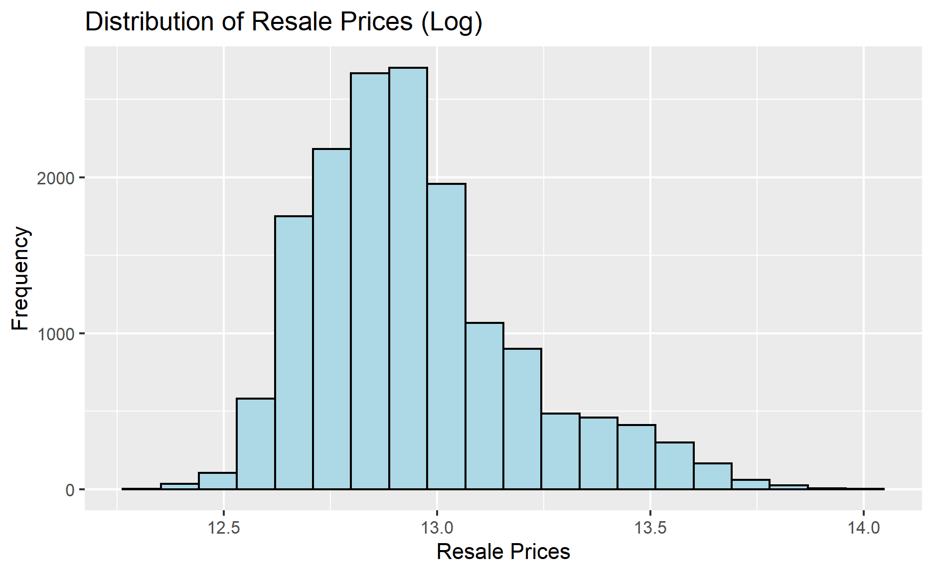
The post-tranformation histogram is relatively less skewed - though the difference isn’t particularly visually significant. Do note that we will still be using RESALE_PRICE in the later parts of our analysis.
We can also use boxplots to see this distribution:
Show code
ggplot(data = resale_sf, aes(x = '', y = PRICE)) +
geom_boxplot() +
labs(x='', y='Resale Prices')
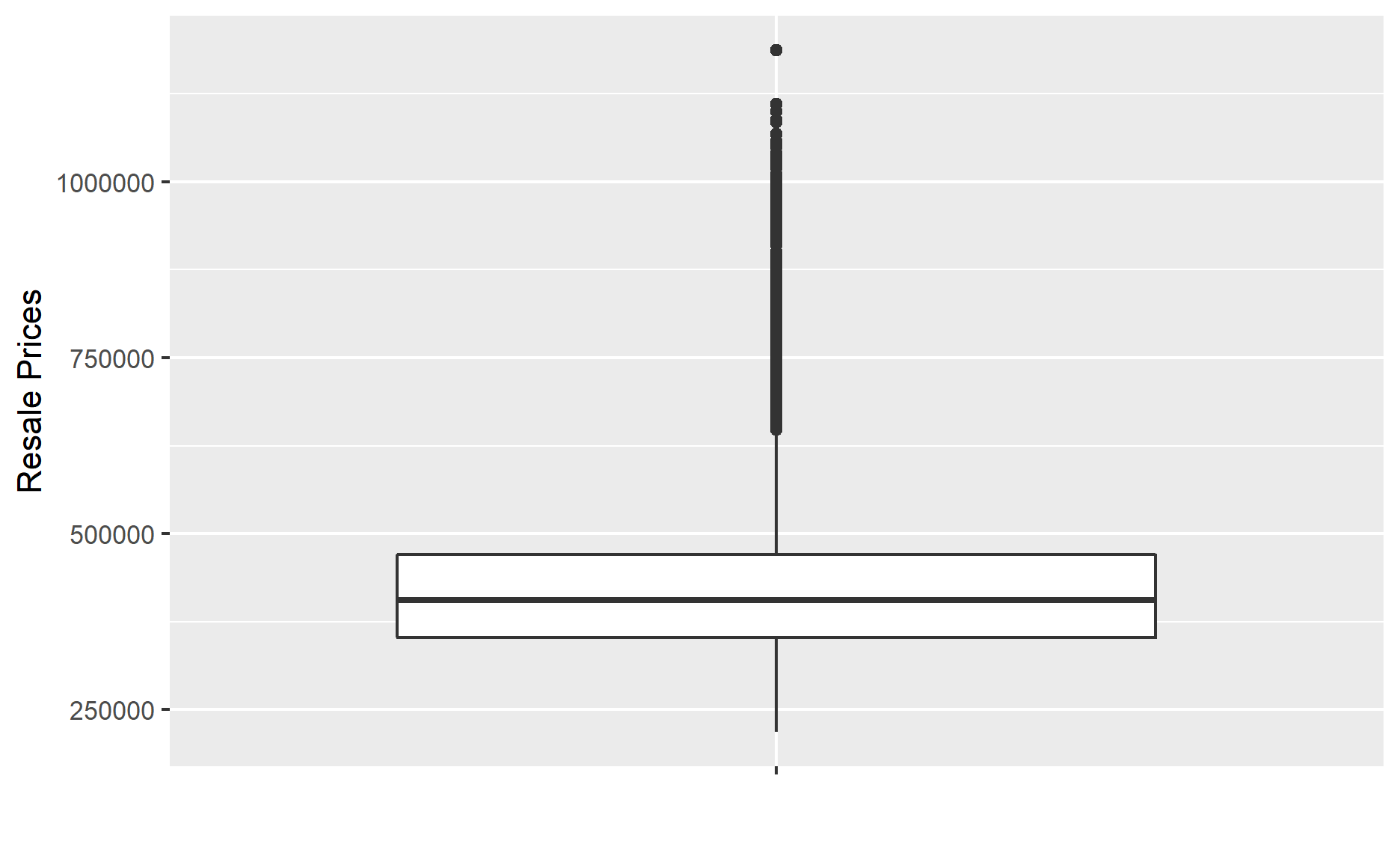
This distribution is in line with our summary statistics from earlier, with our first quartile being at 352800, the median at 405000 and the third quartile being 470000. Generally, most buildings seem to fall within 375000 and 500000 - though as we can see, there’s quite a number of outliers on the high end, with the biggest outlier being over twice the amount of our third quartile at 1186888.
5.2 Multiple histogram plots of distribution of locational factors
We should also take a look at the distribution of our locational factors:
Show code
AREA_SQM <- ggplot(data = resale_sf, aes(x = `AREA_SQ`)) +
geom_histogram(bins=20, color="black", fill = 'lightblue')
LEASE_YRS <- ggplot(data = resale_sf, aes(x = `LEASE_Y`)) +
geom_histogram(bins=20, color="black", fill = 'lightblue')
PROX_CBD <- ggplot(data = resale_sf, aes(x = `PROX_CB`)) +
geom_histogram(bins=20, color="black", fill = 'lightblue')
PROX_CHILDCARE <- ggplot(data = resale_sf, aes(x = `PROX_CH`)) +
geom_histogram(bins=20, color="black", fill = 'lightblue')
PROX_ELDERCARE <- ggplot(data = resale_sf, aes(x = `PROX_EL`)) +
geom_histogram(bins=20, color="black", fill = 'lightblue')
PROX_HAWKER <- ggplot(data = resale_sf, aes(x = `PROX_HA`)) +
geom_histogram(bins=20, color="black", fill = 'lightblue')
PROX_MRT <- ggplot(data = resale_sf, aes(x = `PROX_MR`)) +
geom_histogram(bins=20, color="black", fill = 'lightblue')
PROX_PARK <- ggplot(data = resale_sf, aes(x = `PROX_PA`)) +
geom_histogram(bins=20, color="black", fill = 'lightblue')
PROX_TOPPRISCH <- ggplot(data = resale_sf, aes(x = `PROX_TO`)) +
geom_histogram(bins=20, color="black", fill = 'lightblue')
PROX_MALL <- ggplot(data = resale_sf, aes(x = `PROX_MA`)) +
geom_histogram(bins=20, color="black", fill = 'lightblue')
PROX_SPRMKT <- ggplot(data = resale_sf, aes(x = `PROX_SP`)) +
geom_histogram(bins=20, color="black", fill = 'lightblue')
PROX_HOSPITAL <- ggplot(data = resale_sf, aes(x = `PROX_HO`)) +
geom_histogram(bins=20, color="black", fill = 'lightblue')
ggarrange(AREA_SQM, LEASE_YRS, PROX_CBD, PROX_CHILDCARE, PROX_ELDERCARE, PROX_HAWKER, PROX_MRT, PROX_PARK, PROX_TOPPRISCH, PROX_MALL, PROX_SPRMKT, PROX_HOSPITAL, ncol = 3, nrow = 4)
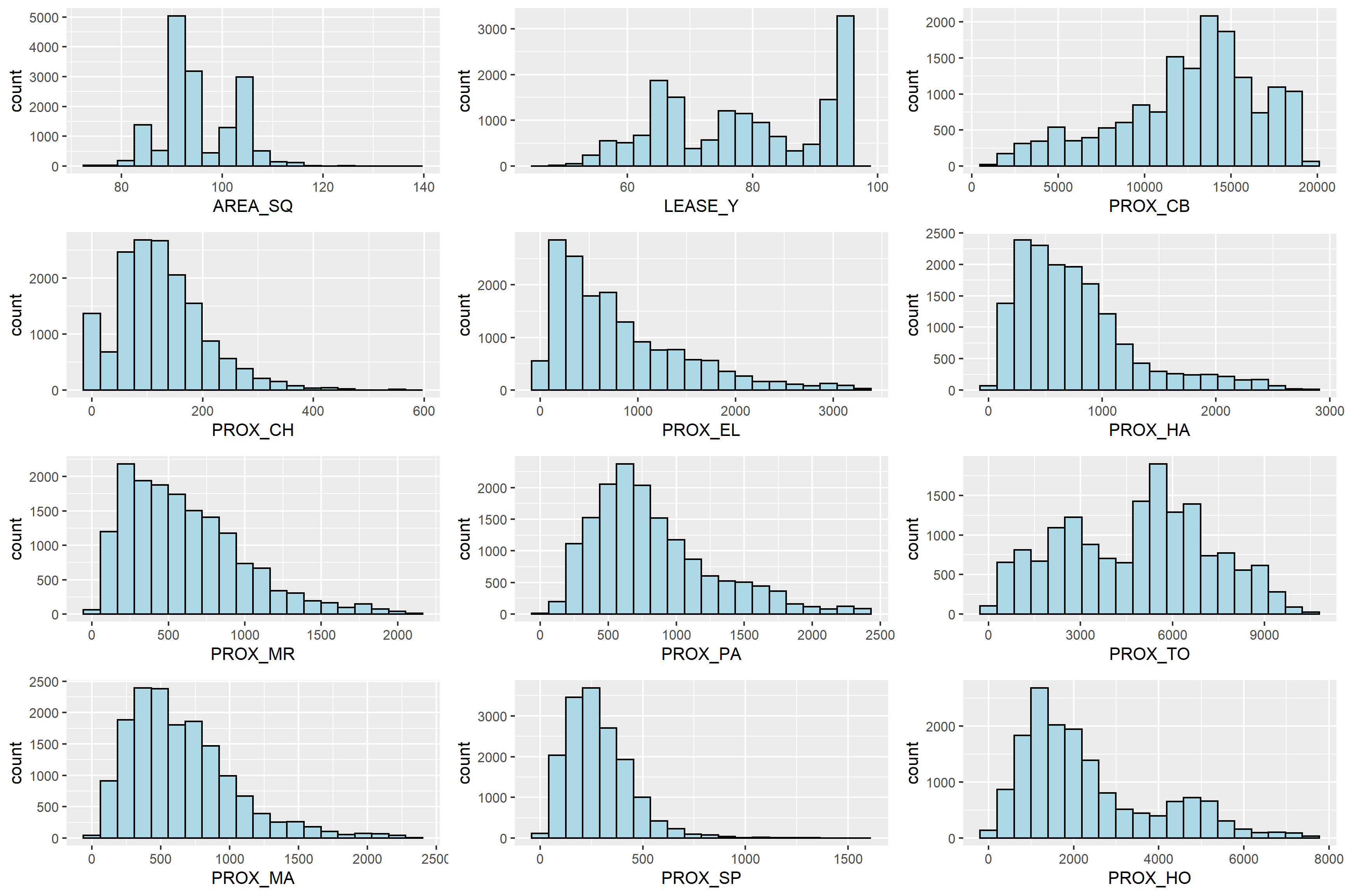
Show code
NUM_CHILDCARE <- ggplot(data = resale_sf, aes(x = `NUM_CHI`)) +
geom_histogram(bins=20, color="black", fill = 'lightblue')
NUM_KNDRGTN <- ggplot(data = resale_sf, aes(x = `NUM_KND`)) +
geom_histogram(bins=20, color="black", fill = 'lightblue')
NUM_BUS_STOP <- ggplot(data = resale_sf, aes(x = `NUM_BUS`)) +
geom_histogram(bins=20, color="black", fill = 'lightblue')
NUM_ISP_CLIN <- ggplot(data = resale_sf, aes(x = `NUM_ISP`)) +
geom_histogram(bins=20, color="black", fill = 'lightblue')
NUM_CHAS_CLIN <- ggplot(data = resale_sf, aes(x = `NUM_CHA`)) +
geom_histogram(bins=20, color="black", fill = 'lightblue')
ggarrange(NUM_KNDRGTN, NUM_CHILDCARE, NUM_BUS_STOP, NUM_ISP_CLIN, NUM_CHAS_CLIN, ncol = 2, nrow = 3)
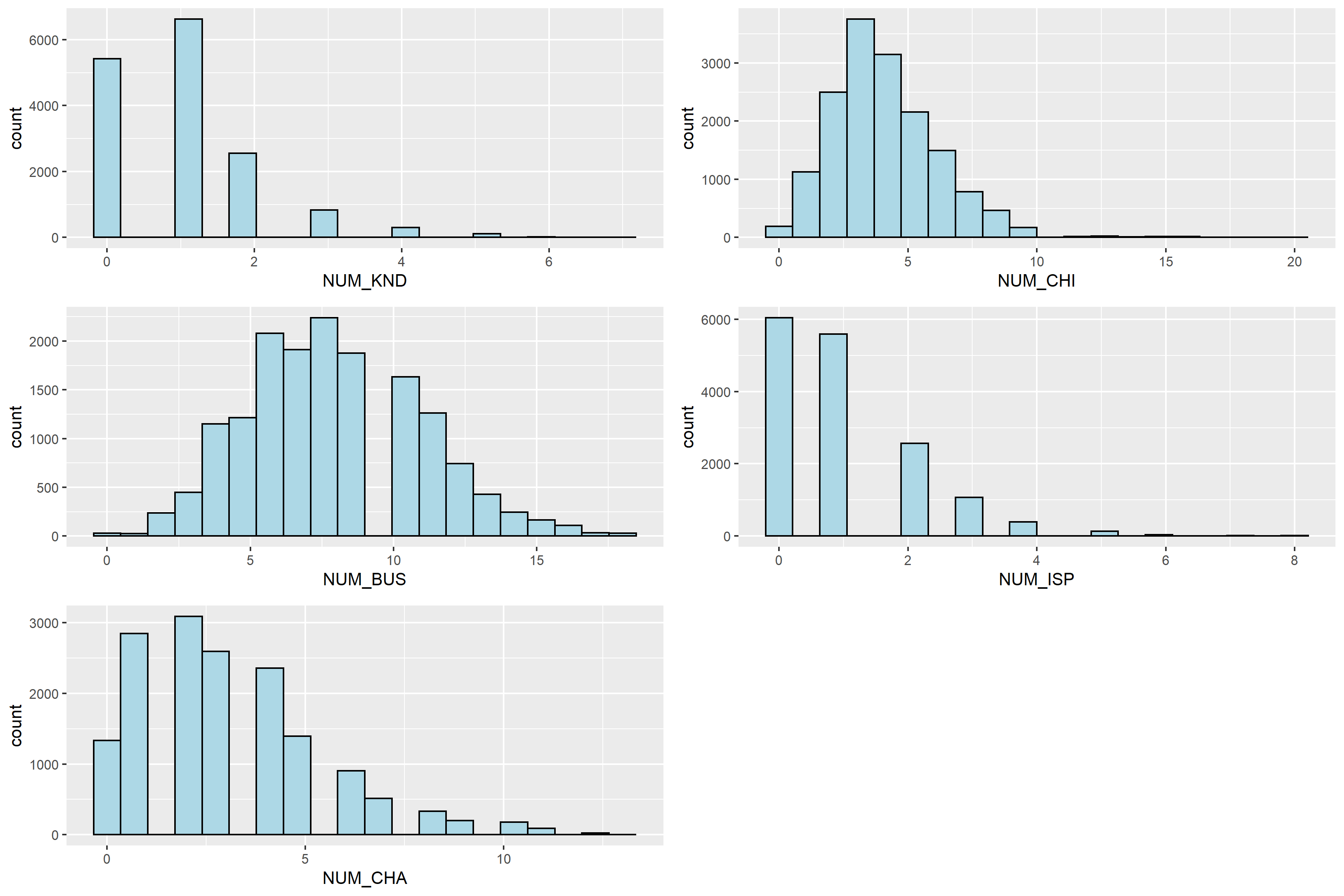
5.3 Statistical Point Map
Let’s create an interactive map that reveals the geospatial distribution of resale prices of 4-room housing units in Singapore:
Show code
tmap_mode("view")
tmap_options(check.and.fix = TRUE)
tm_shape(resale_sf) +
tm_dots(col = "PRICE",
alpha = 0.6,
style="quantile") +
# sets minimum zoom level to 11, sets maximum zoom level to 14
tm_view(set.zoom.limits = c(11,14))
Before moving on to the next section, we’ll revert the R display into plot mode for future visualisations.
Show code
# return tmap mode to plot for future visualisations
tmap_mode("plot")
From the map, we can observe that flats with higher resale prices tend to be more concentrated in the central area of Singapore. Let’s dig a little deeper and check if our hypothesis is correct by looking at the towns with the highest average price:
Show code
Simple feature collection with 10 features and 2 fields
Geometry type: MULTIPOINT
Dimension: XY
Bounding box: xmin: 19863.73 ymin: 28217.39 xmax: 38132.57 ymax: 38389.24
Projected CRS: SVY21 / Singapore TM
Group.1 PRICE geometry
1 CENTRAL AREA 727203.3 MULTIPOINT ((28851.09 28922...
2 QUEENSTOWN 711080.8 MULTIPOINT ((22274.14 31974...
3 BUKIT MERAH 651182.8 MULTIPOINT ((25024.14 28462...
4 BUKIT TIMAH 624068.1 MULTIPOINT ((21224.68 35656...
5 TOA PAYOH 555316.0 MULTIPOINT ((29026.28 34720...
6 KALLANG/WHAMPOA 552847.8 MULTIPOINT ((22917.56 35326...
7 CLEMENTI 549439.8 MULTIPOINT ((19863.73 32474...
8 BISHAN 546857.4 MULTIPOINT ((27638.13 37842...
9 GEYLANG 516142.9 MULTIPOINT ((32789.43 33305...
10 MARINE PARADE 487452.3 MULTIPOINT ((36223.84 31782...We can see that ‘Central Area’ ranks the highest amongst the mean resale price, and with central town Queenstown not far behind. The are other other central towns such as Bishan and Mraine Parade relatively highly too (making the top 10) - indicating a high density of highly-priced housing units that are resold.
6.0 Linear Regression
6.1 Simple Linear Regression
Firstly, let’s build a simple linear regression model with PRICE as our dependent variable and AREA_SQM as our independent variable. In land-scarce Singapore where a plot of land is worth its weight in gold, it would make sense that area of the housing unit is the biggest factor in driving prices up - so let’s test this hypothesis:
Show code
# output: class 'lm' object or class c('mlm', 'lm') multi-response
resale_slr <- lm(formula=PRICE ~ AREA_SQ, data = resale_sf)
We can use the summary() and anova() (short for analysis of variance) functions to obtain and print their related results, like so:
Show code
summary(resale_slr)
Call:
lm(formula = PRICE ~ AREA_SQ, data = resale_sf)
Residuals:
Min 1Q Median 3Q Max
-220708 -79705 -28708 36286 751171
Coefficients:
Estimate Std. Error t value Pr(>|t|)
(Intercept) 528452.8 12797.3 41.294 < 2e-16 ***
AREA_SQ -997.2 134.1 -7.436 1.09e-13 ***
---
Signif. codes: 0 '***' 0.001 '**' 0.01 '*' 0.05 '.' 0.1 ' ' 1
Residual standard error: 120000 on 15851 degrees of freedom
Multiple R-squared: 0.003476, Adjusted R-squared: 0.003413
F-statistic: 55.29 on 1 and 15851 DF, p-value: 1.095e-13The output report reveals that the SELLING_PRICE can be explained by using the formula:
\[ y = 528452.8 + -997.2(area) \]
This is shocking! From our summary output above, we see that our multiple R-squared value is 0.003476, which means that the simple regression model built is able to explain about only 0.3% of the resale prices - a very poor model indeed!
Since our p-value is much smaller than 0.0001, we will reject the null hypothesis that the mean is a good estimator of PRICE. This allows us to infer that the simple linear regression model above is a good estimator of PRICE.
The Coefficients: section of the report reveals that the p-values of both the estimates of the Intercept and AREA_SQ are smaller than 0.001. Within this context, the null hypothesis of the B0 and B1 are equal to 0 will be rejected. As such, we can infer that B0 and B1 are good parameter estimates.
Let’s try visualising the model with a best fit curve:
Show code
ggplot(data=resale_sf,
aes(x=`AREA_SQ`, y=`PRICE`)) +
geom_point() +
geom_smooth(method = lm)
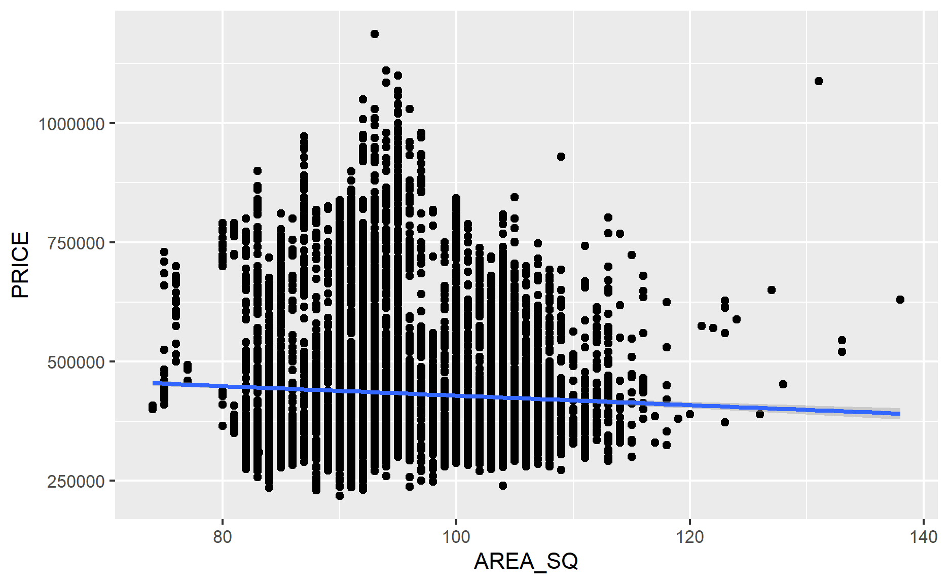
Look at that level of variability - the values of AREA_SQ can barely fit into that straight line. No wonder the model is so poorly fitted. From here, we can conclude that that AREA_SQ is not a good indicator of predicting the PRICE.
6.2 Multiple Linear Regression
6.2.1 Visualising the relationships of the independent variables
Just like in the our Hands-on Exercise 08, before building a multiple regression model, we need to perform correlation analysis so as to ensure that the cluster variables are not highly correlated. “Why?” Well - if you have two variables that are highly correlated (aka collinear) - the concept they represent is effectively similar, which compromises the quality of our model as it becomes skewed towards those collinear variables.
A correlation matrix is commonly used to visualise the relationships between the independent variables: in this section, the corrplot package will be used. Now, let’s try plotting a scatterplot matrix of the relationship between the independent variables in resale_sf. We’ll use the AOE order, which orders the variables by the angular order of eigenvectors.
Show code
resale_nogeom_sf <- resale_sf %>%
st_drop_geometry()
Show code
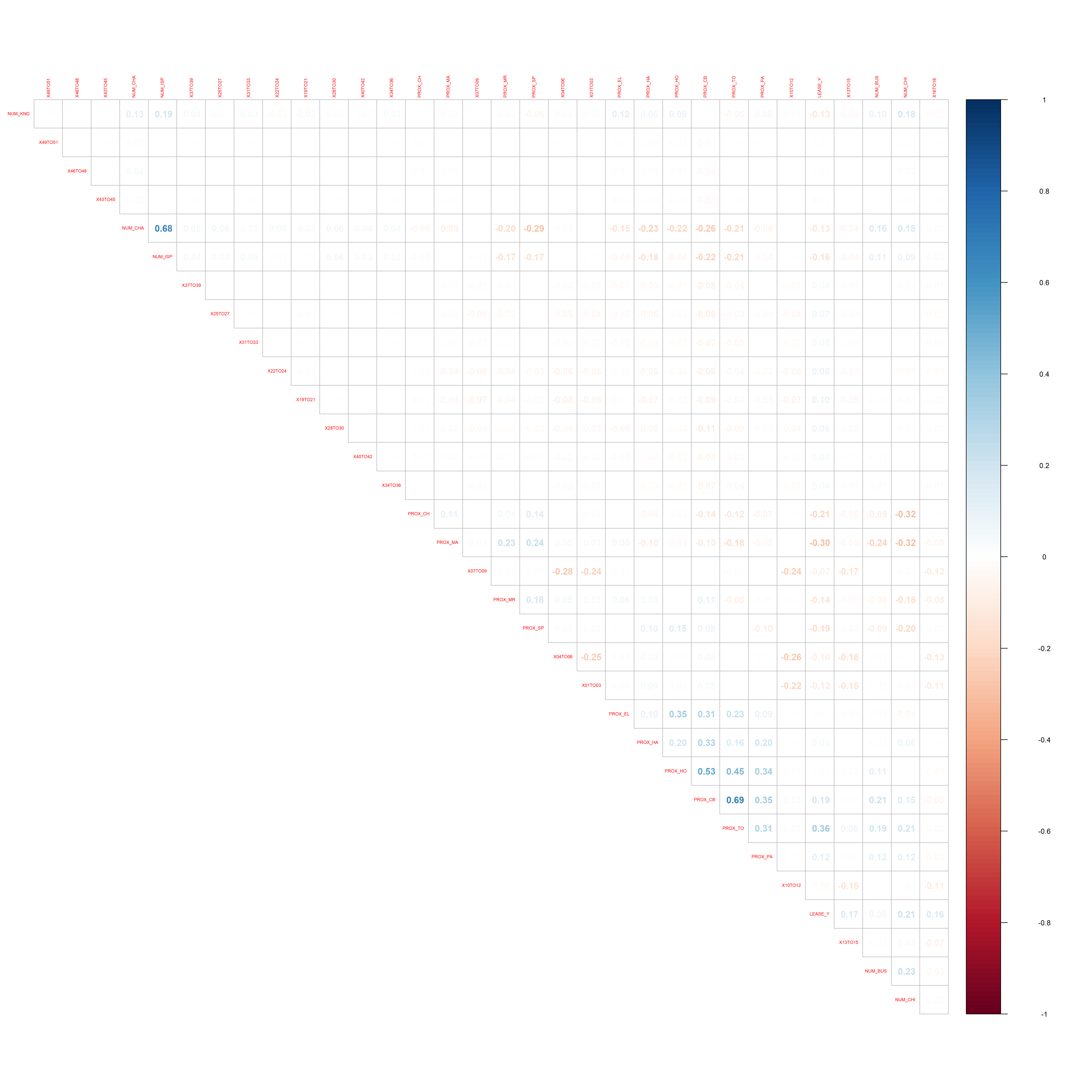
As we can see, there is high positive correlation between NUM_ISP and NUM_CHA, which refers to the clinics that support the Community Health Assistance Scheme and/or have the Integrated Screening Programme. Seeing as a good portion of clinics are government-owned or government-supported, it would make sense for them to have both of these government schemes.
Between the two, we’ll pick NUM_CHA for the CHAS, which subsidises citizens of all ages and is likely to be of more concern to potential houseowners.
Lastly - there is a very high positive correlation between PROX_CB and PROX_TO, representing proximity to the CBD and to Top Primary Schools respectively. This is reflected in reality, where the top primary schools are clustered near to the central region. Between the two, I find the proximity to top primary schools a more interesting and significant factor, on account of the earlier research on how location affects priority for primary school registration. As such, we’ll remove PROX_CB as well.
6.2.2 Building a hedonic pricing model using multiple linear regression method
Show code
resale_mlr <- lm(formula = PRICE ~ AREA_SQ + LEASE_Y +
X01TO03 + X04TO06 + X07TO09 + X10TO12 + X13TO15 + X16TO18 +
X19TO21 + X22TO24 + X25TO27 + X28TO30 + X31TO33 + X34TO36 +
X37TO39 + X40TO42 + X43TO45 + X46TO48 + X49TO51 +
PROX_CH + PROX_EL + PROX_HA + PROX_MR + PROX_PA + PROX_TO +
PROX_MA + PROX_SP + PROX_HO +
NUM_KND + NUM_CHI + NUM_BUS + NUM_CHA,
data = resale_sf)
summary(resale_mlr)
Call:
lm(formula = PRICE ~ AREA_SQ + LEASE_Y + X01TO03 + X04TO06 +
X07TO09 + X10TO12 + X13TO15 + X16TO18 + X19TO21 + X22TO24 +
X25TO27 + X28TO30 + X31TO33 + X34TO36 + X37TO39 + X40TO42 +
X43TO45 + X46TO48 + X49TO51 + PROX_CH + PROX_EL + PROX_HA +
PROX_MR + PROX_PA + PROX_TO + PROX_MA + PROX_SP + PROX_HO +
NUM_KND + NUM_CHI + NUM_BUS + NUM_CHA, data = resale_sf)
Residuals:
Min 1Q Median 3Q Max
-238779 -44346 -7930 34521 633175
Coefficients:
Estimate Std. Error t value Pr(>|t|)
(Intercept) 1.614e+05 1.595e+04 10.124 < 2e-16 ***
AREA_SQ 1.927e+03 8.436e+01 22.838 < 2e-16 ***
LEASE_Y 4.450e+03 5.538e+01 80.353 < 2e-16 ***
X01TO03 -8.048e+04 1.231e+04 -6.539 6.37e-11 ***
X04TO06 -6.074e+04 1.227e+04 -4.950 7.51e-07 ***
X07TO09 -4.513e+04 1.225e+04 -3.683 0.000231 ***
X10TO12 -3.651e+04 1.225e+04 -2.980 0.002884 **
X13TO15 -2.829e+04 1.227e+04 -2.305 0.021178 *
X16TO18 -9.879e+03 1.242e+04 -0.796 0.426318
X19TO21 1.824e+04 1.286e+04 1.419 0.155913
X22TO24 1.591e+04 1.299e+04 1.224 0.220786
X25TO27 7.103e+04 1.375e+04 5.167 2.41e-07 ***
X28TO30 1.526e+05 1.419e+04 10.752 < 2e-16 ***
X31TO33 1.564e+05 1.706e+04 9.168 < 2e-16 ***
X34TO36 1.618e+05 1.786e+04 9.057 < 2e-16 ***
X37TO39 2.339e+05 1.757e+04 13.310 < 2e-16 ***
X40TO42 2.833e+05 1.949e+04 14.537 < 2e-16 ***
X43TO45 4.032e+05 4.272e+04 9.437 < 2e-16 ***
X46TO48 4.499e+05 4.274e+04 10.526 < 2e-16 ***
X49TO51 5.163e+05 5.161e+04 10.004 < 2e-16 ***
PROX_CH 4.540e+01 7.617e+00 5.960 2.57e-09 ***
PROX_EL -2.151e+01 9.316e-01 -23.087 < 2e-16 ***
PROX_HA -3.776e+01 1.191e+00 -31.705 < 2e-16 ***
PROX_MR -4.394e+01 1.556e+00 -28.238 < 2e-16 ***
PROX_PA -1.714e+01 1.407e+00 -12.180 < 2e-16 ***
PROX_TO -2.207e+01 3.066e-01 -71.985 < 2e-16 ***
PROX_MA -1.646e+01 1.695e+00 -9.714 < 2e-16 ***
PROX_SP -1.926e+01 4.049e+00 -4.755 2.00e-06 ***
PROX_HO 6.834e-01 4.502e-01 1.518 0.129042
NUM_KND 7.693e+03 5.974e+02 12.877 < 2e-16 ***
NUM_CHI -5.998e+03 3.389e+02 -17.701 < 2e-16 ***
NUM_BUS -1.427e+03 2.090e+02 -6.826 9.05e-12 ***
NUM_CHA 4.352e+03 2.910e+02 14.954 < 2e-16 ***
---
Signif. codes: 0 '***' 0.001 '**' 0.01 '*' 0.05 '.' 0.1 ' ' 1
Residual standard error: 70860 on 15820 degrees of freedom
Multiple R-squared: 0.6532, Adjusted R-squared: 0.6525
F-statistic: 931 on 32 and 15820 DF, p-value: < 2.2e-16As we can clearly see, not all the independent variables are statistically significant, and said variables should be removed. The variables I’ve identified as insignificant are X16TO18, X19TO21, X22TO24 and surprisingly, PROX_HO.
Show code
resale_mlr1 <- lm(formula = PRICE ~ AREA_SQ + LEASE_Y +
X01TO03 + X04TO06 + X07TO09 + X10TO12 + X13TO15 + X25TO27 + X28TO30 +
X31TO33 + X34TO36 + X37TO39 + X40TO42 + X43TO45 + X46TO48 + X49TO51 +
PROX_CH + PROX_EL + PROX_HA + PROX_MR +
PROX_PA + PROX_TO + PROX_MA + PROX_SP +
NUM_KND + NUM_CHI + NUM_BUS + NUM_CHA,
data = resale_sf)
ols_regress(resale_mlr1)
Model Summary
----------------------------------------------------------------------
R 0.808 RMSE 70956.925
R-Squared 0.652 Coef. Var 16.366
Adj. R-Squared 0.651 MSE 5034885272.222
Pred R-Squared 0.650 MAE 52523.942
----------------------------------------------------------------------
RMSE: Root Mean Square Error
MSE: Mean Square Error
MAE: Mean Absolute Error
ANOVA
--------------------------------------------------------------------------------
Sum of
Squares DF Mean Square F Sig.
--------------------------------------------------------------------------------
Regression 1.493393e+14 28 5.333546e+12 1059.318 0.0000
Residual 7.967202e+13 15824 5034885272.222
Total 2.290113e+14 15852
--------------------------------------------------------------------------------
Parameter Estimates
-----------------------------------------------------------------------------------------------------
model Beta Std. Error Std. Beta t Sig lower upper
-----------------------------------------------------------------------------------------------------
(Intercept) 160806.759 10406.162 15.453 0.000 140409.497 181204.022
AREA_SQ 1944.817 84.062 0.115 23.136 0.000 1780.046 2109.588
LEASE_Y 4452.321 55.026 0.476 80.913 0.000 4344.464 4560.178
X01TO03 -80934.487 2470.645 -0.256 -32.758 0.000 -85777.233 -76091.741
X04TO06 -61211.352 2365.400 -0.215 -25.878 0.000 -65847.805 -56574.900
X07TO09 -45612.104 2382.315 -0.154 -19.146 0.000 -50281.712 -40942.496
X10TO12 -36989.878 2409.565 -0.120 -15.351 0.000 -41712.899 -32266.857
X13TO15 -28828.154 2659.106 -0.072 -10.841 0.000 -34040.305 -23616.003
X25TO27 70563.149 6705.651 0.052 10.523 0.000 57419.309 83706.988
X28TO30 152227.005 7850.823 0.094 19.390 0.000 136838.498 167615.512
X31TO33 155603.706 12033.583 0.062 12.931 0.000 132016.512 179190.901
X34TO36 160712.169 13149.122 0.058 12.222 0.000 134938.392 186485.946
X37TO39 232940.593 12750.821 0.087 18.269 0.000 207947.530 257933.655
X40TO42 282312.799 15288.787 0.087 18.465 0.000 252345.034 312280.563
X43TO45 401857.558 41031.026 0.046 9.794 0.000 321432.073 482283.043
X46TO48 448612.460 41053.882 0.051 10.927 0.000 368142.175 529082.745
X49TO51 515081.779 50245.673 0.048 10.251 0.000 416594.536 613569.022
PROX_CH 45.538 7.624 0.030 5.973 0.000 30.595 60.482
PROX_EL -21.109 0.903 -0.116 -23.374 0.000 -22.879 -19.339
PROX_HA -38.132 1.190 -0.164 -32.055 0.000 -40.463 -35.800
PROX_MR -43.932 1.557 -0.141 -28.220 0.000 -46.983 -40.880
PROX_PA -16.437 1.365 -0.061 -12.041 0.000 -19.112 -13.761
PROX_TO -22.001 0.288 -0.439 -76.403 0.000 -22.566 -21.437
PROX_MA -16.942 1.694 -0.054 -10.001 0.000 -20.262 -13.621
PROX_SP -18.266 4.012 -0.024 -4.552 0.000 -26.131 -10.401
NUM_KND 7721.312 596.131 0.065 12.952 0.000 6552.827 8889.797
NUM_CHI -6138.794 337.747 -0.101 -18.176 0.000 -6800.815 -5476.772
NUM_BUS -1396.796 209.034 -0.034 -6.682 0.000 -1806.526 -987.066
NUM_CHA 4390.253 290.126 0.083 15.132 0.000 3821.573 4958.933
-----------------------------------------------------------------------------------------------------6.3 Testing LR Assumptions
There are 4 assumptions that must be met before we perform regression on geographical data:
- Test of multicollinearity: ensure that the variables are not highly correlated
- Test of non-linearity: the relationship between the dependent variable and independent variables should be approximately linear
- Testing for normality assumption: The residuals are assumed to be normally distributed
- Test for spatial autocorrelation
6.3.1 Checking for multicollinearity
We’ll test for signs of multicollinearity with the ols_vif_tol() function of our olsrr package. In general, if the VIF value is less than 5, then there is usually no sign/possibility of correlations.
Show code
ols_vif_tol(resale_mlr1)
Variables Tolerance VIF
1 AREA_SQ 0.8900449 1.123539
2 LEASE_Y 0.6364966 1.571100
3 X01TO03 0.3599011 2.778541
4 X04TO06 0.3198524 3.126442
5 X07TO09 0.3401095 2.940229
6 X10TO12 0.3622126 2.760810
7 X13TO15 0.5033970 1.986504
8 X25TO27 0.9174562 1.089970
9 X28TO30 0.9334564 1.071287
10 X31TO33 0.9680203 1.033036
11 X34TO36 0.9725175 1.028259
12 X37TO39 0.9697076 1.031239
13 X40TO42 0.9804466 1.019943
14 X43TO45 0.9970703 1.002938
15 X46TO48 0.9959604 1.004056
16 X49TO51 0.9972798 1.002728
17 PROX_CH 0.8648215 1.156308
18 PROX_EL 0.8869688 1.127435
19 PROX_HA 0.8442889 1.184429
20 PROX_MR 0.8805382 1.135669
21 PROX_PA 0.8464960 1.181341
22 PROX_TO 0.6666714 1.499989
23 PROX_MA 0.7531833 1.327698
24 PROX_SP 0.7973261 1.254192
25 NUM_KND 0.8768119 1.140495
26 NUM_CHI 0.7146305 1.399324
27 NUM_BUS 0.8592054 1.163866
28 NUM_CHA 0.7268085 1.375878Since the VIF of the independent variables is less than 10, we can safely conclude that there are no signs of multicollinearity amongst the independent variables. 😄
6.3.2 Test for Non-Linearity
In addition to testing for multicollinearity, we also need to test the assumption that linearity and additivity of the relationship between dependent and independent variables when performing multiple linear regression.
We’ll perform the linearity assumption test with the ols_plot_resid_fit() function:
Show code
ols_plot_resid_fit(resale_mlr1)
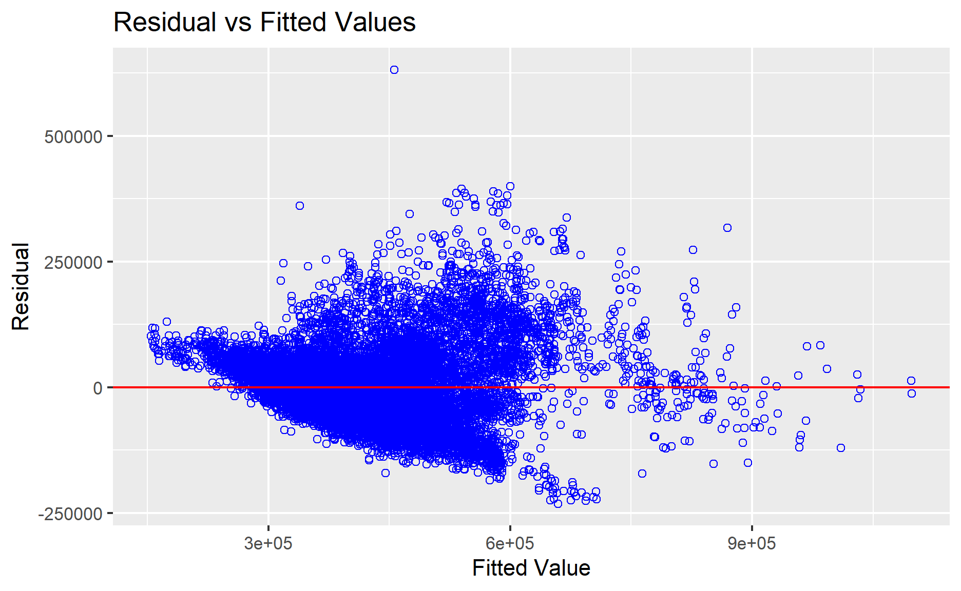
For most part, our data points are scattered around the 0 line (though there are a few outliers). However, it is still within range of tolernace, thus we can safely conclude that the relationships between the dependent variable and independent variables are linear.
6.3.3 Test for Normality Assumption
Next, we’ll perform the normality assumption test with the ols_plot_resid_hist() function:
Show code
ols_plot_resid_hist(resale_mlr1)
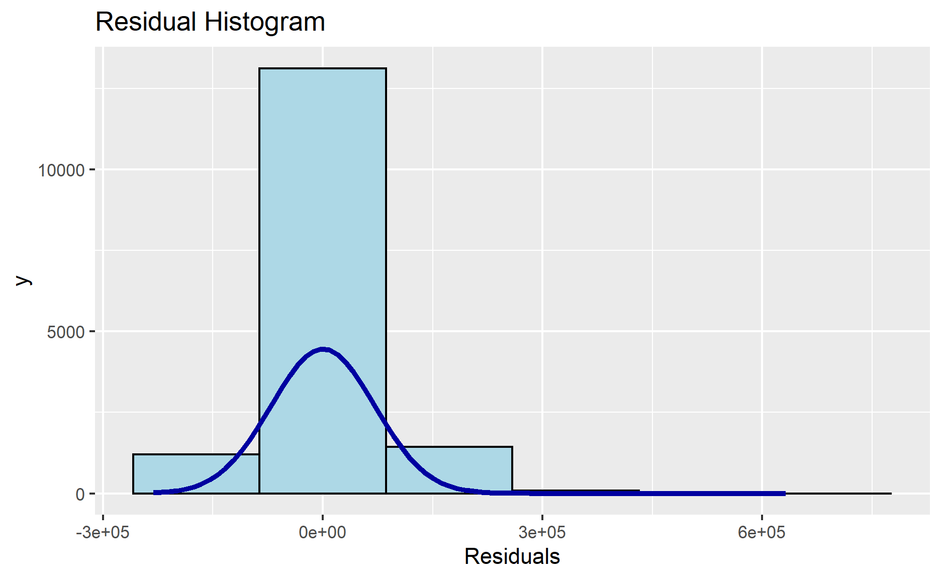
As we can see, the residual of the multiple linear regression model (i.e. resale_mlr1) resembles a normal distribution.
6.3.4 Testing for Spatial Autocorrelation
Since hedonic model we aim to build is using geographically referenced attributes, it is important for us to visualize the residual of the hedonic pricing model. In order to the perform spatial autocorrelation test, we’l need to convert resale_mlr1 simple into a SpatialPointsDataFrame.
Show code
mlr_output <- as.data.frame(resale_mlr1$residuals)
resale_res_sf <- cbind(resale_sf,
resale_mlr1$residuals) %>%
rename(`MLR_RES` = `resale_mlr1.residuals`)
Show code
# convert from a simple features object to a SpatialPointsDataFrame
# due to requirements of using the spdep package
resale_sp <- as_Spatial(resale_res_sf)
resale_sp
class : SpatialPointsDataFrame
features : 15853
extent : 11597.31, 42623.63, 28217.39, 48741.06 (xmin, xmax, ymin, ymax)
crs : +proj=tmerc +lat_0=1.36666666666667 +lon_0=103.833333333333 +k=1 +x_0=28001.642 +y_0=38744.572 +ellps=WGS84 +towgs84=0,0,0,0,0,0,0 +units=m +no_defs
variables : 43
names : PRICE, month, town, flt_typ, block, strt_nm, AREA_SQ, flt_mdl, ls_cmm_, LEASE_Y, X01TO03, X07TO09, X04TO06, X10TO12, X13TO15, ...
min values : 218000, 2019-01, ANG MO KIO, 4 ROOM, 1, ADMIRALTY DR, 74, Adjoined flat, 1967, 45.5, 0, 0, 0, 0, 0, ...
max values : 1186888, 2020-09, YISHUN, 4 ROOM, 9B, YUNG SHENG RD, 138, Type S1, 2018, 97, 1, 1, 1, 1, 1, ... Now, let’s display the distribution of the residuals on an interactive map:
Show code
tmap_mode("view")
tm_shape(mpsz_sf)+
tm_polygons(alpha = 0.4) +
tm_shape(resale_sp) +
tm_dots(col = "MLR_RES",
alpha = 0.6,
style="quantile") +
tm_view(set.zoom.limits = c(11,14))
Show code
#switch back to 'plot' before continuing
tmap_mode("plot")
There ARE indeed signs of spatial autocorrelation. To proof that our observation is indeed true, the Moran’s I test will be performed.
6.3.5 Moran I’s Test
Firstly, let’s compute the distance-based weight matrix by using the dnearneigh() function of the spdep package.
Show code
nb <- dnearneigh(coordinates(resale_sp), 0, 1500, longlat = FALSE)
summary(nb)
Neighbour list object:
Number of regions: 15853
Number of nonzero links: 10145534
Percentage nonzero weights: 4.036937
Average number of links: 639.9757
Link number distribution:
2 7 14 25 26 31 32 46 56 57 60 65 68 69
3 1 14 15 5 4 2 47 4 4 5 2 4 1
71 72 75 78 85 86 88 89 90 96 97 99 100 103
12 1 1 77 2 1 5 4 3 5 3 8 6 2
106 109 110 112 115 117 118 119 120 121 122 123 124 125
2 5 8 3 6 7 3 6 8 4 7 19 9 57
126 128 130 131 132 133 134 135 136 137 138 139 141 142
17 30 2 15 13 10 4 3 5 9 21 13 9 13
143 144 145 146 147 148 149 150 151 152 153 154 155 156
3 3 6 6 19 4 1 3 21 18 14 6 5 10
157 159 160 161 163 164 166 167 168 169 170 171 172 173
10 17 7 4 15 9 11 5 4 8 3 8 9 5
174 175 176 177 178 179 180 181 182 183 184 185 186 187
12 22 15 27 8 18 7 3 13 8 8 28 30 17
188 189 190 191 192 193 194 195 196 197 198 199 200 201
6 7 3 7 9 7 7 3 4 7 18 8 21 29
202 203 204 205 206 207 208 209 211 212 213 214 215 216
13 3 12 14 3 10 20 5 2 8 9 10 21 7
217 218 219 220 221 222 223 224 225 226 227 228 229 230
1 6 11 21 28 40 1 13 10 4 20 22 5 14
231 232 233 234 235 236 237 238 239 240 241 242 243 244
11 10 4 13 38 14 3 18 7 37 21 5 10 13
245 246 247 248 249 250 251 252 253 254 255 256 257 258
8 8 21 17 9 5 35 17 9 14 9 16 11 7
259 260 261 262 263 264 265 266 267 268 269 270 271 272
8 4 13 11 19 12 14 17 16 40 6 7 37 54
273 274 275 276 277 278 279 280 281 282 283 284 285 286
19 16 20 28 62 2 45 53 28 17 31 19 25 45
287 288 289 290 291 292 293 294 295 296 297 298 299 300
51 44 24 46 52 25 30 51 14 9 35 17 15 26
301 302 303 304 305 306 307 308 309 310 311 312 313 314
41 26 14 32 23 17 21 7 3 20 9 10 26 18
315 316 317 318 319 320 321 322 323 324 325 326 327 328
10 17 43 15 22 26 26 27 32 26 26 30 26 32
329 330 331 332 333 334 335 336 337 338 339 340 341 342
18 44 6 17 23 14 30 10 47 21 21 36 23 1
343 344 345 346 347 348 349 350 351 352 353 354 355 356
35 20 12 10 31 41 29 9 21 39 19 17 27 17
357 358 359 360 361 362 363 364 365 366 367 368 369 370
19 23 31 24 13 35 19 10 29 26 43 10 22 28
371 372 373 374 375 376 377 378 379 380 381 382 383 384
22 10 41 24 11 62 8 23 16 16 22 16 9 17
385 386 387 388 389 390 391 392 393 394 395 396 397 398
39 20 38 31 21 17 16 31 4 15 39 13 21 22
399 400 401 402 403 404 405 406 407 408 409 410 411 412
21 20 26 20 17 28 16 6 14 24 20 14 21 34
413 414 415 416 417 418 419 420 421 422 423 424 425 426
6 21 22 10 12 76 8 20 18 49 34 18 26 27
427 428 429 430 431 432 433 434 435 436 437 438 439 440
28 23 20 23 11 28 37 11 33 22 20 22 23 11
441 442 443 444 445 446 447 448 449 450 451 452 453 454
23 13 6 6 25 10 19 34 15 21 9 29 26 10
455 456 457 458 459 460 461 462 463 464 465 466 467 468
27 24 70 16 15 8 14 12 9 40 13 5 22 25
469 470 471 472 473 474 475 476 477 478 479 480 481 482
3 35 13 21 14 12 18 13 28 24 25 29 18 6
483 484 485 486 487 488 489 490 491 492 493 494 495 496
10 14 14 18 12 23 20 15 10 7 27 18 7 8
497 498 499 500 501 502 503 504 505 506 507 508 509 510
14 2 8 10 10 16 21 8 34 25 19 18 15 43
511 512 513 514 515 516 517 518 519 520 521 522 523 524
20 29 12 6 15 9 4 13 2 4 16 8 13 10
525 526 527 528 529 530 531 532 533 534 535 536 537 538
11 8 20 36 17 17 17 7 17 14 11 22 5 6
539 540 541 542 543 544 545 546 548 549 550 551 553 554
9 4 7 10 14 17 17 14 7 12 16 16 11 9
555 556 557 558 559 560 561 562 563 564 565 566 567 568
8 16 15 7 28 8 4 5 23 15 16 22 21 22
569 570 571 572 573 574 575 576 577 578 579 580 581 582
14 6 23 4 23 28 24 17 22 4 16 14 4 10
583 584 585 586 587 588 589 590 591 592 593 594 595 596
10 9 16 15 10 24 17 18 22 20 5 16 9 19
597 598 599 600 601 602 603 604 605 606 607 608 609 610
12 9 16 14 14 3 18 6 18 13 9 10 25 14
611 612 613 614 615 616 617 618 619 620 621 622 623 624
31 5 2 12 24 3 32 15 5 6 11 6 11 16
625 626 627 628 629 630 631 632 633 634 635 636 637 638
3 14 23 4 6 7 18 7 12 20 15 10 11 7
639 640 641 642 643 644 645 646 647 648 649 650 651 652
5 8 15 17 2 10 33 2 17 6 17 24 8 10
653 654 655 656 657 658 659 660 661 663 664 665 666 667
11 6 5 6 7 23 10 7 5 10 1 4 3 6
668 669 670 671 672 673 674 675 676 677 678 679 680 681
19 21 5 2 9 20 10 3 5 6 13 24 6 7
682 683 684 685 686 687 688 689 690 691 692 693 694 695
30 53 3 4 8 3 7 24 6 19 10 10 9 12
696 697 698 699 700 701 702 703 704 705 706 707 708 709
12 24 3 18 9 7 10 19 7 17 4 8 3 4
710 711 712 713 714 715 716 717 718 719 720 721 722 723
30 7 2 8 13 34 8 23 10 3 17 4 12 10
725 726 727 728 729 730 731 732 733 734 735 736 737 738
2 17 7 2 6 24 1 2 2 6 7 1 11 7
739 740 741 742 743 744 745 746 747 748 749 750 751 752
4 13 9 4 13 16 12 18 22 26 19 16 5 5
753 754 755 756 757 758 760 761 762 763 764 765 766 767
13 4 16 21 4 22 4 9 8 3 24 25 29 1
768 769 770 771 772 773 774 775 776 777 778 779 780 781
26 7 19 3 22 13 13 18 21 14 6 34 33 19
782 784 785 786 787 788 789 790 791 792 793 794 795 796
13 3 12 15 4 5 7 15 24 16 4 11 3 54
797 798 799 800 802 803 804 805 806 807 808 809 810 812
16 16 9 11 23 3 20 13 20 21 30 35 12 19
813 814 815 816 817 818 819 820 821 822 823 824 825 826
7 13 5 34 26 20 28 15 5 13 13 7 8 3
827 828 829 830 831 832 833 834 835 836 837 838 839 840
29 12 15 12 11 3 31 15 24 9 31 6 5 11
841 842 843 844 845 846 847 848 849 850 851 852 853 854
17 10 3 21 9 15 17 13 29 9 19 5 34 10
855 856 857 858 859 860 861 862 863 864 865 866 867 868
8 15 15 4 1 26 32 7 6 3 18 22 7 2
869 870 871 872 873 874 875 876 877 878 879 880 881 882
5 4 2 1 5 16 18 10 2 9 1 4 7 14
883 884 885 886 887 888 889 890 891 892 893 894 895 896
14 10 5 20 1 13 13 1 17 5 9 11 9 7
897 898 899 900 901 902 903 904 905 906 907 908 909 910
12 15 9 7 10 10 35 9 6 8 2 8 10 18
911 914 915 916 917 918 919 920 921 922 923 924 925 926
2 7 3 5 32 11 12 10 26 4 10 6 4 24
927 928 929 930 932 933 934 935 936 937 938 940 941 942
8 4 2 6 5 15 13 1 32 1 10 3 8 3
943 945 946 947 948 949 950 951 952 955 957 959 960 961
2 1 1 1 10 4 20 8 6 1 2 14 2 5
963 964 965 966 967 968 969 971 972 973 974 975 976 977
11 18 2 18 6 4 2 21 2 16 1 4 4 35
979 980 981 982 984 985 986 988 991 992 993 996 997 998
14 3 8 5 4 1 3 31 10 1 2 10 1 21
999 1000 1001 1003 1005 1006 1007 1008 1010 1011 1012 1013 1014 1015
10 2 3 8 16 9 7 2 4 7 3 6 15 13
1016 1017 1018 1019 1020 1021 1022 1023 1024 1025 1026 1027 1028 1029
11 11 19 6 9 6 10 11 1 16 2 1 3 18
1032 1033 1034 1035 1037 1038 1039 1040 1041 1042 1043 1044 1045 1046
18 6 3 9 3 2 10 9 5 7 9 11 6 9
1048 1050 1051 1052 1053 1055 1056 1057 1058 1059 1060 1061 1064 1065
18 4 3 5 23 1 7 15 5 4 1 3 4 15
1066 1071 1076 1077 1078 1079 1081 1082 1085 1086 1087 1088 1089 1091
1 9 9 4 4 7 1 11 3 5 19 7 3 14
1092 1094 1097 1099 1102 1104 1107 1109 1110 1111 1113 1114 1116 1117
3 11 8 5 6 5 4 2 22 2 3 9 3 13
1118 1119 1121 1123 1124 1128 1129 1132 1133 1134 1135 1136 1137 1138
4 9 8 10 4 11 25 2 7 8 2 21 7 9
1139 1140 1142 1143 1144 1145 1146 1147 1148 1149 1150 1152 1153 1155
15 21 7 6 4 14 4 5 5 13 3 8 15 2
1156 1157 1158 1159 1160 1161 1162 1163 1164 1165 1168 1169 1170 1172
1 15 1 9 5 15 4 15 14 8 25 12 20 7
1173 1174 1175 1177 1178 1180 1182 1183 1185 1186 1187 1188 1191 1192
41 12 2 9 7 3 6 8 8 11 20 6 5 2
1194 1195 1196 1197 1198 1200 1201 1203 1204 1205 1206 1207 1209 1210
6 7 8 13 16 9 10 4 4 13 1 14 7 7
1214 1215 1216 1217 1218 1219 1220 1221 1222 1223 1224 1225 1226 1227
10 6 11 2 36 40 9 22 16 5 13 7 7 11
1228 1230 1231 1233 1234 1235 1237 1238 1239 1240 1241 1242 1243 1245
4 13 10 23 19 2 25 3 1 8 4 11 8 1
1246 1249 1250 1251 1254 1256 1257 1259 1260 1261 1262 1263 1264 1265
2 1 5 7 4 6 2 2 10 1 7 3 1 2
1266 1267 1269 1270 1271 1274 1275 1276 1277 1278 1279 1280 1281 1282
19 12 6 3 3 1 3 6 4 22 5 7 1 7
1283 1284 1285 1286 1287 1288 1289 1291 1292 1296 1297 1298 1300 1301
2 1 10 6 2 3 4 4 5 12 3 6 5 3
1302 1303 1304 1305 1306 1307 1308 1310 1311 1312 1313 1315 1318 1319
6 4 22 12 12 5 2 21 5 6 1 17 1 5
1320 1321 1322 1324 1325 1326 1327 1328 1329 1331 1332 1333 1335 1336
3 3 6 7 16 1 1 8 1 10 11 6 16 13
1337 1338 1339 1340 1341 1342 1343 1344 1346 1347 1349 1352 1355 1356
10 1 12 9 13 22 18 5 1 17 6 8 8 29
1357 1358 1362 1363 1364 1365 1367 1368 1370 1372 1373 1375 1376 1377
6 2 27 5 2 1 1 12 12 13 6 11 4 11
1378 1379 1380 1381 1382 1383 1385 1387 1388 1390 1391 1392 1395 1397
6 19 3 2 5 16 1 7 10 24 5 3 5 13
1399 1400 1401 1402 1404 1405 1408 1409 1410 1414 1417 1420 1422 1423
5 1 11 9 3 9 6 5 17 5 17 3 3 2
1427 1428 1429 1431 1433 1435 1436 1439 1442 1443 1446 1450 1451 1452
1 1 1 1 1 1 10 2 4 19 6 2 1 8
1454 1457 1458 1463 1464 1466 1467 1469 1470 1471 1473 1478 1479 1480
11 1 4 1 2 5 2 1 7 2 2 1 3 9
1483 1484 1486 1487 1488 1491 1492 1495 1496 1498 1509 1517 1518 1520
1 2 11 1 1 7 2 1 20 1 2 3 3 2
1526 1530 1531 1533 1537 1538 1539 1542 1545 1547 1552 1555 1557 1559
6 4 12 1 3 2 3 1 2 7 4 2 3 2
1563 1567 1571 1577 1578 1582 1583 1584 1587 1592 1594 1602 1608 1612
15 1 2 4 1 8 3 1 3 6 2 9 1 1
1614 1616 1620 1628 1630 1638 1644 1645 1669 1678 1687 1691 1699 1718
2 2 2 2 16 1 3 4 1 1 1 1 5 1
1728 1731 1735 1746 1748 1758 1762 1767 1768 1793 1799 1802 1810 1845
1 3 5 3 2 3 4 4 1 4 5 4 1 3
1868 1875 1913 1942 1956
3 1 2 5 4
3 least connected regions:
3083 4737 5544 with 2 links
4 most connected regions:
3250 8144 12521 13498 with 1956 linksWe’ll convert the output neighbours lists (i.e. nb) into a spatial weights with the nb2listw() function:
Show code
nb_lw <- nb2listw(nb, style = 'W')
summary(nb_lw)
Characteristics of weights list object:
Neighbour list object:
Number of regions: 15853
Number of nonzero links: 10145534
Percentage nonzero weights: 4.036937
Average number of links: 639.9757
Link number distribution:
2 7 14 25 26 31 32 46 56 57 60 65 68 69
3 1 14 15 5 4 2 47 4 4 5 2 4 1
71 72 75 78 85 86 88 89 90 96 97 99 100 103
12 1 1 77 2 1 5 4 3 5 3 8 6 2
106 109 110 112 115 117 118 119 120 121 122 123 124 125
2 5 8 3 6 7 3 6 8 4 7 19 9 57
126 128 130 131 132 133 134 135 136 137 138 139 141 142
17 30 2 15 13 10 4 3 5 9 21 13 9 13
143 144 145 146 147 148 149 150 151 152 153 154 155 156
3 3 6 6 19 4 1 3 21 18 14 6 5 10
157 159 160 161 163 164 166 167 168 169 170 171 172 173
10 17 7 4 15 9 11 5 4 8 3 8 9 5
174 175 176 177 178 179 180 181 182 183 184 185 186 187
12 22 15 27 8 18 7 3 13 8 8 28 30 17
188 189 190 191 192 193 194 195 196 197 198 199 200 201
6 7 3 7 9 7 7 3 4 7 18 8 21 29
202 203 204 205 206 207 208 209 211 212 213 214 215 216
13 3 12 14 3 10 20 5 2 8 9 10 21 7
217 218 219 220 221 222 223 224 225 226 227 228 229 230
1 6 11 21 28 40 1 13 10 4 20 22 5 14
231 232 233 234 235 236 237 238 239 240 241 242 243 244
11 10 4 13 38 14 3 18 7 37 21 5 10 13
245 246 247 248 249 250 251 252 253 254 255 256 257 258
8 8 21 17 9 5 35 17 9 14 9 16 11 7
259 260 261 262 263 264 265 266 267 268 269 270 271 272
8 4 13 11 19 12 14 17 16 40 6 7 37 54
273 274 275 276 277 278 279 280 281 282 283 284 285 286
19 16 20 28 62 2 45 53 28 17 31 19 25 45
287 288 289 290 291 292 293 294 295 296 297 298 299 300
51 44 24 46 52 25 30 51 14 9 35 17 15 26
301 302 303 304 305 306 307 308 309 310 311 312 313 314
41 26 14 32 23 17 21 7 3 20 9 10 26 18
315 316 317 318 319 320 321 322 323 324 325 326 327 328
10 17 43 15 22 26 26 27 32 26 26 30 26 32
329 330 331 332 333 334 335 336 337 338 339 340 341 342
18 44 6 17 23 14 30 10 47 21 21 36 23 1
343 344 345 346 347 348 349 350 351 352 353 354 355 356
35 20 12 10 31 41 29 9 21 39 19 17 27 17
357 358 359 360 361 362 363 364 365 366 367 368 369 370
19 23 31 24 13 35 19 10 29 26 43 10 22 28
371 372 373 374 375 376 377 378 379 380 381 382 383 384
22 10 41 24 11 62 8 23 16 16 22 16 9 17
385 386 387 388 389 390 391 392 393 394 395 396 397 398
39 20 38 31 21 17 16 31 4 15 39 13 21 22
399 400 401 402 403 404 405 406 407 408 409 410 411 412
21 20 26 20 17 28 16 6 14 24 20 14 21 34
413 414 415 416 417 418 419 420 421 422 423 424 425 426
6 21 22 10 12 76 8 20 18 49 34 18 26 27
427 428 429 430 431 432 433 434 435 436 437 438 439 440
28 23 20 23 11 28 37 11 33 22 20 22 23 11
441 442 443 444 445 446 447 448 449 450 451 452 453 454
23 13 6 6 25 10 19 34 15 21 9 29 26 10
455 456 457 458 459 460 461 462 463 464 465 466 467 468
27 24 70 16 15 8 14 12 9 40 13 5 22 25
469 470 471 472 473 474 475 476 477 478 479 480 481 482
3 35 13 21 14 12 18 13 28 24 25 29 18 6
483 484 485 486 487 488 489 490 491 492 493 494 495 496
10 14 14 18 12 23 20 15 10 7 27 18 7 8
497 498 499 500 501 502 503 504 505 506 507 508 509 510
14 2 8 10 10 16 21 8 34 25 19 18 15 43
511 512 513 514 515 516 517 518 519 520 521 522 523 524
20 29 12 6 15 9 4 13 2 4 16 8 13 10
525 526 527 528 529 530 531 532 533 534 535 536 537 538
11 8 20 36 17 17 17 7 17 14 11 22 5 6
539 540 541 542 543 544 545 546 548 549 550 551 553 554
9 4 7 10 14 17 17 14 7 12 16 16 11 9
555 556 557 558 559 560 561 562 563 564 565 566 567 568
8 16 15 7 28 8 4 5 23 15 16 22 21 22
569 570 571 572 573 574 575 576 577 578 579 580 581 582
14 6 23 4 23 28 24 17 22 4 16 14 4 10
583 584 585 586 587 588 589 590 591 592 593 594 595 596
10 9 16 15 10 24 17 18 22 20 5 16 9 19
597 598 599 600 601 602 603 604 605 606 607 608 609 610
12 9 16 14 14 3 18 6 18 13 9 10 25 14
611 612 613 614 615 616 617 618 619 620 621 622 623 624
31 5 2 12 24 3 32 15 5 6 11 6 11 16
625 626 627 628 629 630 631 632 633 634 635 636 637 638
3 14 23 4 6 7 18 7 12 20 15 10 11 7
639 640 641 642 643 644 645 646 647 648 649 650 651 652
5 8 15 17 2 10 33 2 17 6 17 24 8 10
653 654 655 656 657 658 659 660 661 663 664 665 666 667
11 6 5 6 7 23 10 7 5 10 1 4 3 6
668 669 670 671 672 673 674 675 676 677 678 679 680 681
19 21 5 2 9 20 10 3 5 6 13 24 6 7
682 683 684 685 686 687 688 689 690 691 692 693 694 695
30 53 3 4 8 3 7 24 6 19 10 10 9 12
696 697 698 699 700 701 702 703 704 705 706 707 708 709
12 24 3 18 9 7 10 19 7 17 4 8 3 4
710 711 712 713 714 715 716 717 718 719 720 721 722 723
30 7 2 8 13 34 8 23 10 3 17 4 12 10
725 726 727 728 729 730 731 732 733 734 735 736 737 738
2 17 7 2 6 24 1 2 2 6 7 1 11 7
739 740 741 742 743 744 745 746 747 748 749 750 751 752
4 13 9 4 13 16 12 18 22 26 19 16 5 5
753 754 755 756 757 758 760 761 762 763 764 765 766 767
13 4 16 21 4 22 4 9 8 3 24 25 29 1
768 769 770 771 772 773 774 775 776 777 778 779 780 781
26 7 19 3 22 13 13 18 21 14 6 34 33 19
782 784 785 786 787 788 789 790 791 792 793 794 795 796
13 3 12 15 4 5 7 15 24 16 4 11 3 54
797 798 799 800 802 803 804 805 806 807 808 809 810 812
16 16 9 11 23 3 20 13 20 21 30 35 12 19
813 814 815 816 817 818 819 820 821 822 823 824 825 826
7 13 5 34 26 20 28 15 5 13 13 7 8 3
827 828 829 830 831 832 833 834 835 836 837 838 839 840
29 12 15 12 11 3 31 15 24 9 31 6 5 11
841 842 843 844 845 846 847 848 849 850 851 852 853 854
17 10 3 21 9 15 17 13 29 9 19 5 34 10
855 856 857 858 859 860 861 862 863 864 865 866 867 868
8 15 15 4 1 26 32 7 6 3 18 22 7 2
869 870 871 872 873 874 875 876 877 878 879 880 881 882
5 4 2 1 5 16 18 10 2 9 1 4 7 14
883 884 885 886 887 888 889 890 891 892 893 894 895 896
14 10 5 20 1 13 13 1 17 5 9 11 9 7
897 898 899 900 901 902 903 904 905 906 907 908 909 910
12 15 9 7 10 10 35 9 6 8 2 8 10 18
911 914 915 916 917 918 919 920 921 922 923 924 925 926
2 7 3 5 32 11 12 10 26 4 10 6 4 24
927 928 929 930 932 933 934 935 936 937 938 940 941 942
8 4 2 6 5 15 13 1 32 1 10 3 8 3
943 945 946 947 948 949 950 951 952 955 957 959 960 961
2 1 1 1 10 4 20 8 6 1 2 14 2 5
963 964 965 966 967 968 969 971 972 973 974 975 976 977
11 18 2 18 6 4 2 21 2 16 1 4 4 35
979 980 981 982 984 985 986 988 991 992 993 996 997 998
14 3 8 5 4 1 3 31 10 1 2 10 1 21
999 1000 1001 1003 1005 1006 1007 1008 1010 1011 1012 1013 1014 1015
10 2 3 8 16 9 7 2 4 7 3 6 15 13
1016 1017 1018 1019 1020 1021 1022 1023 1024 1025 1026 1027 1028 1029
11 11 19 6 9 6 10 11 1 16 2 1 3 18
1032 1033 1034 1035 1037 1038 1039 1040 1041 1042 1043 1044 1045 1046
18 6 3 9 3 2 10 9 5 7 9 11 6 9
1048 1050 1051 1052 1053 1055 1056 1057 1058 1059 1060 1061 1064 1065
18 4 3 5 23 1 7 15 5 4 1 3 4 15
1066 1071 1076 1077 1078 1079 1081 1082 1085 1086 1087 1088 1089 1091
1 9 9 4 4 7 1 11 3 5 19 7 3 14
1092 1094 1097 1099 1102 1104 1107 1109 1110 1111 1113 1114 1116 1117
3 11 8 5 6 5 4 2 22 2 3 9 3 13
1118 1119 1121 1123 1124 1128 1129 1132 1133 1134 1135 1136 1137 1138
4 9 8 10 4 11 25 2 7 8 2 21 7 9
1139 1140 1142 1143 1144 1145 1146 1147 1148 1149 1150 1152 1153 1155
15 21 7 6 4 14 4 5 5 13 3 8 15 2
1156 1157 1158 1159 1160 1161 1162 1163 1164 1165 1168 1169 1170 1172
1 15 1 9 5 15 4 15 14 8 25 12 20 7
1173 1174 1175 1177 1178 1180 1182 1183 1185 1186 1187 1188 1191 1192
41 12 2 9 7 3 6 8 8 11 20 6 5 2
1194 1195 1196 1197 1198 1200 1201 1203 1204 1205 1206 1207 1209 1210
6 7 8 13 16 9 10 4 4 13 1 14 7 7
1214 1215 1216 1217 1218 1219 1220 1221 1222 1223 1224 1225 1226 1227
10 6 11 2 36 40 9 22 16 5 13 7 7 11
1228 1230 1231 1233 1234 1235 1237 1238 1239 1240 1241 1242 1243 1245
4 13 10 23 19 2 25 3 1 8 4 11 8 1
1246 1249 1250 1251 1254 1256 1257 1259 1260 1261 1262 1263 1264 1265
2 1 5 7 4 6 2 2 10 1 7 3 1 2
1266 1267 1269 1270 1271 1274 1275 1276 1277 1278 1279 1280 1281 1282
19 12 6 3 3 1 3 6 4 22 5 7 1 7
1283 1284 1285 1286 1287 1288 1289 1291 1292 1296 1297 1298 1300 1301
2 1 10 6 2 3 4 4 5 12 3 6 5 3
1302 1303 1304 1305 1306 1307 1308 1310 1311 1312 1313 1315 1318 1319
6 4 22 12 12 5 2 21 5 6 1 17 1 5
1320 1321 1322 1324 1325 1326 1327 1328 1329 1331 1332 1333 1335 1336
3 3 6 7 16 1 1 8 1 10 11 6 16 13
1337 1338 1339 1340 1341 1342 1343 1344 1346 1347 1349 1352 1355 1356
10 1 12 9 13 22 18 5 1 17 6 8 8 29
1357 1358 1362 1363 1364 1365 1367 1368 1370 1372 1373 1375 1376 1377
6 2 27 5 2 1 1 12 12 13 6 11 4 11
1378 1379 1380 1381 1382 1383 1385 1387 1388 1390 1391 1392 1395 1397
6 19 3 2 5 16 1 7 10 24 5 3 5 13
1399 1400 1401 1402 1404 1405 1408 1409 1410 1414 1417 1420 1422 1423
5 1 11 9 3 9 6 5 17 5 17 3 3 2
1427 1428 1429 1431 1433 1435 1436 1439 1442 1443 1446 1450 1451 1452
1 1 1 1 1 1 10 2 4 19 6 2 1 8
1454 1457 1458 1463 1464 1466 1467 1469 1470 1471 1473 1478 1479 1480
11 1 4 1 2 5 2 1 7 2 2 1 3 9
1483 1484 1486 1487 1488 1491 1492 1495 1496 1498 1509 1517 1518 1520
1 2 11 1 1 7 2 1 20 1 2 3 3 2
1526 1530 1531 1533 1537 1538 1539 1542 1545 1547 1552 1555 1557 1559
6 4 12 1 3 2 3 1 2 7 4 2 3 2
1563 1567 1571 1577 1578 1582 1583 1584 1587 1592 1594 1602 1608 1612
15 1 2 4 1 8 3 1 3 6 2 9 1 1
1614 1616 1620 1628 1630 1638 1644 1645 1669 1678 1687 1691 1699 1718
2 2 2 2 16 1 3 4 1 1 1 1 5 1
1728 1731 1735 1746 1748 1758 1762 1767 1768 1793 1799 1802 1810 1845
1 3 5 3 2 3 4 4 1 4 5 4 1 3
1868 1875 1913 1942 1956
3 1 2 5 4
3 least connected regions:
3083 4737 5544 with 2 links
4 most connected regions:
3250 8144 12521 13498 with 1956 links
Weights style: W
Weights constants summary:
n nn S0 S1 S2
W 15853 251317609 15853 79.65655 63911.4Lastly, to perform Moran’s I test for residual spatial autocorrelation, we’ll use the lm.morantest() function:
Show code
lm.morantest(resale_mlr1, nb_lw)
Global Moran I for regression residuals
data:
model: lm(formula = PRICE ~ AREA_SQ + LEASE_Y + X01TO03 +
X04TO06 + X07TO09 + X10TO12 + X13TO15 + X25TO27 + X28TO30 +
X31TO33 + X34TO36 + X37TO39 + X40TO42 + X43TO45 + X46TO48 +
X49TO51 + PROX_CH + PROX_EL + PROX_HA + PROX_MR + PROX_PA +
PROX_TO + PROX_MA + PROX_SP + NUM_KND + NUM_CHI + NUM_BUS +
NUM_CHA, data = resale_sf)
weights: nb_lw
Moran I statistic standard deviate = 1005, p-value < 2.2e-16
alternative hypothesis: greater
sample estimates:
Observed Moran I Expectation Variance
5.125732e-01 -3.769831e-04 2.605246e-07 The Global Moran’s I test for residual spatial autocorrelation shows that its p-value is less than the alpha value of 0.05. Hence, we will reject the null hypothesis that the residuals are randomly distributed.
Since the Observed Global Moran I is greater than 0, we can infer that the residuals resemble cluster distribution.
7.0 Building Hedonic Pricing Models using GWmodel
7.1 Building Adaptive Bandwidth GWR Model
7.1.1 Computing the adaptive bandwidth
We will first use bw.gwr() to determine the recommended data point to use
Show code
bw_adaptive <- bw.gwr(formula = PRICE ~ AREA_SQ + LEASE_Y +
PROX_CH + PROX_EL + PROX_HA + PROX_MR +
PROX_PA + PROX_TO + PROX_MA + PROX_SP +
NUM_KND + NUM_CHI + NUM_BUS + NUM_CHA,
data=resale_sp, approach="CV", kernel="gaussian",
adaptive=TRUE, longlat=FALSE)
Take a cup of tea and have a break, it will take a few minutes.
-----A kind suggestion from GWmodel development group
Adaptive bandwidth: 9805 CV score: 8.804379e+13
Adaptive bandwidth: 6068 CV score: 7.988997e+13
Adaptive bandwidth: 3757 CV score: 7.121513e+13
Adaptive bandwidth: 2330 CV score: 6.03039e+13
Adaptive bandwidth: 1446 CV score: 4.571792e+13
Adaptive bandwidth: 902 CV score: 3.450122e+13
Adaptive bandwidth: 563 CV score: 2.770476e+13
Adaptive bandwidth: 356 CV score: 2.40023e+13
Adaptive bandwidth: 225 CV score: 2.104461e+13
Adaptive bandwidth: 147 CV score: 1.878976e+13
Adaptive bandwidth: 96 CV score: 1.705054e+13
Adaptive bandwidth: 67 CV score: 1.601827e+13
Adaptive bandwidth: 46 CV score: 1.666599e+13
Adaptive bandwidth: 76 CV score: 1.62724e+13
Adaptive bandwidth: 57 CV score: 1.565215e+13
Adaptive bandwidth: 55 CV score: 1.560372e+13
Adaptive bandwidth: 49 CV score: 1.645738e+13
Adaptive bandwidth: 53 CV score: 1.551122e+13
Adaptive bandwidth: 58 CV score: 1.568018e+13
Adaptive bandwidth: 56 CV score: 1.563509e+13
Adaptive bandwidth: 57 CV score: 1.565215e+13
Adaptive bandwidth: 56 CV score: 1.563509e+13
Adaptive bandwidth: 56 CV score: 1.563509e+13
Adaptive bandwidth: 55 CV score: 1.560372e+13
Adaptive bandwidth: 55 CV score: 1.560372e+13
Adaptive bandwidth: 54 CV score: 1.554991e+13
Adaptive bandwidth: 54 CV score: 1.554991e+13
Adaptive bandwidth: 53 CV score: 1.551122e+13 The result shows that number of recommended data point, which we will use for generating the adaptive bandwidth GWR model.
7.1.2 Constructing the adaptive bandwidth gwr model
Now, we can calibrate the gwr-based hedonic pricing model by using adaptive bandwidth and gaussian kernel:
Show code
gwr_adaptive <- gwr.basic(formula = PRICE ~ AREA_SQ + LEASE_Y +
PROX_CH + PROX_EL + PROX_HA + PROX_MR +
PROX_PA + PROX_TO + PROX_MA + PROX_SP +
NUM_KND + NUM_CHI + NUM_BUS + NUM_CHA,
data=resale_sp, bw=bw_adaptive,
kernel = 'gaussian', adaptive=TRUE, longlat = FALSE)
Let’s display the model output:
Show code
gwr_adaptive
***********************************************************************
* Package GWmodel *
***********************************************************************
Program starts at: 2021-11-08 07:25:23
Call:
gwr.basic(formula = PRICE ~ AREA_SQ + LEASE_Y + PROX_CH + PROX_EL +
PROX_HA + PROX_MR + PROX_PA + PROX_TO + PROX_MA + PROX_SP +
NUM_KND + NUM_CHI + NUM_BUS + NUM_CHA, data = resale_sp,
bw = bw_adaptive, kernel = "gaussian", adaptive = TRUE, longlat = FALSE)
Dependent (y) variable: PRICE
Independent variables: AREA_SQ LEASE_Y PROX_CH PROX_EL PROX_HA PROX_MR PROX_PA PROX_TO PROX_MA PROX_SP NUM_KND NUM_CHI NUM_BUS NUM_CHA
Number of data points: 15853
***********************************************************************
* Results of Global Regression *
***********************************************************************
Call:
lm(formula = formula, data = data)
Residuals:
Min 1Q Median 3Q Max
-204669 -50385 -10227 37061 644643
Coefficients:
Estimate Std. Error t value Pr(>|t|)
(Intercept) 94800.4727 11331.7137 8.366 < 2e-16 ***
AREA_SQ 1539.4637 93.3382 16.493 < 2e-16 ***
LEASE_Y 5377.0498 58.0850 92.572 < 2e-16 ***
PROX_CH 62.3452 8.4913 7.342 2.20e-13 ***
PROX_EL -22.3751 1.0065 -22.231 < 2e-16 ***
PROX_HA -43.6140 1.3230 -32.965 < 2e-16 ***
PROX_MR -48.2755 1.7303 -27.899 < 2e-16 ***
PROX_PA -15.3845 1.5207 -10.117 < 2e-16 ***
PROX_TO -24.2807 0.3176 -76.453 < 2e-16 ***
PROX_MA -20.5461 1.8879 -10.883 < 2e-16 ***
PROX_SP -5.3371 4.4682 -1.194 0.232
NUM_KND 10033.2866 662.0961 15.154 < 2e-16 ***
NUM_CHI -6724.6081 376.1937 -17.875 < 2e-16 ***
NUM_BUS -1753.9176 232.9782 -7.528 5.42e-14 ***
NUM_CHA 6042.3100 321.6884 18.783 < 2e-16 ***
---Significance stars
Signif. codes: 0 '***' 0.001 '**' 0.01 '*' 0.05 '.' 0.1 ' ' 1
Residual standard error: 79160 on 15838 degrees of freedom
Multiple R-squared: 0.5666
Adjusted R-squared: 0.5662
F-statistic: 1479 on 14 and 15838 DF, p-value: < 2.2e-16
***Extra Diagnostic information
Residual sum of squares: 9.925189e+13
Sigma(hat): 79129.98
AIC: 402626
AICc: 402626
BIC: 387050.5
***********************************************************************
* Results of Geographically Weighted Regression *
***********************************************************************
*********************Model calibration information*********************
Kernel function: gaussian
Adaptive bandwidth: 53 (number of nearest neighbours)
Regression points: the same locations as observations are used.
Distance metric: Euclidean distance metric is used.
****************Summary of GWR coefficient estimates:******************
Min. 1st Qu. Median 3rd Qu.
Intercept -4.8566e+08 -3.7550e+05 -5.4334e+04 2.3577e+05
AREA_SQ -6.1295e+04 1.5058e+03 2.3418e+03 3.7743e+03
LEASE_Y -2.1343e+04 3.1470e+03 4.9859e+03 7.1725e+03
PROX_CH -2.3866e+03 -5.1347e+01 -9.1952e+00 3.3733e+01
PROX_EL -2.2748e+05 -4.9837e+01 3.5052e+00 5.2180e+01
PROX_HA -7.6736e+04 -5.6941e+01 7.4294e-01 7.9462e+01
PROX_MR -1.0424e+06 -1.3096e+02 -6.0634e+01 -5.5427e-01
PROX_PA -1.0776e+05 -6.3938e+01 -2.2847e+00 4.9159e+01
PROX_TO -3.8150e+04 -6.9121e+01 -1.1384e+01 3.7388e+01
PROX_MA -4.7978e+04 -7.6306e+01 -1.6072e+01 5.4808e+01
PROX_SP -3.8018e+04 -6.1332e+01 -8.0665e+00 5.3076e+01
NUM_KND -3.3811e+05 -6.7604e+03 -6.7678e+02 4.5801e+03
NUM_CHI -9.6538e+04 -2.6455e+03 2.4231e+02 3.2534e+03
NUM_BUS -5.7231e+04 -2.3204e+03 -1.3636e+02 1.7308e+03
NUM_CHA -1.6928e+05 -2.2174e+03 1.6018e+02 2.4711e+03
Max.
Intercept 3.5672e+08
AREA_SQ 4.9388e+04
LEASE_Y 3.1976e+04
PROX_CH 5.1225e+03
PROX_EL 6.1945e+04
PROX_HA 1.2373e+06
PROX_MR 2.1681e+04
PROX_PA 6.2849e+04
PROX_TO 9.5105e+04
PROX_MA 2.5224e+05
PROX_SP 1.1319e+04
NUM_KND 1.0252e+06
NUM_CHI 1.8275e+05
NUM_BUS 1.3905e+05
NUM_CHA 6.1610e+05
************************Diagnostic information*************************
Number of data points: 15853
Effective number of parameters (2trace(S) - trace(S'S)): 1873.456
Effective degrees of freedom (n-2trace(S) + trace(S'S)): 13979.54
AICc (GWR book, Fotheringham, et al. 2002, p. 61, eq 2.33): 372973.8
AIC (GWR book, Fotheringham, et al. 2002,GWR p. 96, eq. 4.22): 371119.8
BIC (GWR book, Fotheringham, et al. 2002,GWR p. 61, eq. 2.34): 368500.7
Residual sum of squares: 1.237911e+13
R-square value: 0.9459454
Adjusted R-square value: 0.9387008
***********************************************************************
Program stops at: 2021-11-08 07:29:09 From this, we can see that the adjusted r-square of the gwr significantly better than the global multiple linear regression model!
7.2 Visualising GWR Output
7.2.1 Converting SDF into sf data.frame
Show code
resale_sf_adaptive <- st_as_sf(gwr_adaptive$SDF) %>%
st_transform(crs=3414)
gwr_adaptive_output <- as.data.frame(gwr_adaptive$SDF)
resale_sf_adaptive <- cbind(resale_res_sf,
as.matrix(gwr_adaptive_output))
glimpse(resale_sf_adaptive)
Rows: 15,853
Columns: 97
$ PRICE <dbl> 330000, 360000, 370000, 375000, 380000, 380000~
$ month <chr> "2019-01", "2019-01", "2019-01", "2019-01", "2~
$ town <chr> "ANG MO KIO", "ANG MO KIO", "ANG MO KIO", "ANG~
$ flt_typ <chr> "4 ROOM", "4 ROOM", "4 ROOM", "4 ROOM", "4 ROO~
$ block <chr> "204", "175", "543", "118", "411", "546", "428~
$ strt_nm <chr> "ANG MO KIO AVE 3", "ANG MO KIO AVE 4", "ANG M~
$ AREA_SQ <dbl> 92, 91, 92, 99, 92, 92, 92, 92, 93, 91, 91, 98~
$ flt_mdl <chr> "New Generation", "New Generation", "New Gener~
$ ls_cmm_ <dbl> 1977, 1981, 1981, 1978, 1979, 1981, 1978, 1982~
$ LEASE_Y <dbl> 57.00, 61.50, 61.08, 58.33, 59.58, 61.00, 58.8~
$ X01TO03 <dbl> 1, 0, 1, 0, 0, 0, 0, 0, 0, 0, 0, 0, 0, 0, 0, 0~
$ X07TO09 <dbl> 0, 1, 0, 0, 0, 0, 1, 0, 0, 1, 1, 1, 0, 1, 0, 0~
$ X04TO06 <dbl> 0, 0, 0, 1, 1, 0, 0, 1, 0, 0, 0, 0, 0, 0, 1, 0~
$ X10TO12 <dbl> 0, 0, 0, 0, 0, 1, 0, 0, 1, 0, 0, 0, 1, 0, 0, 0~
$ X13TO15 <dbl> 0, 0, 0, 0, 0, 0, 0, 0, 0, 0, 0, 0, 0, 0, 0, 1~
$ X25TO27 <dbl> 0, 0, 0, 0, 0, 0, 0, 0, 0, 0, 0, 0, 0, 0, 0, 0~
$ X19TO21 <dbl> 0, 0, 0, 0, 0, 0, 0, 0, 0, 0, 0, 0, 0, 0, 0, 0~
$ X16TO18 <dbl> 0, 0, 0, 0, 0, 0, 0, 0, 0, 0, 0, 0, 0, 0, 0, 0~
$ X28TO30 <dbl> 0, 0, 0, 0, 0, 0, 0, 0, 0, 0, 0, 0, 0, 0, 0, 0~
$ X31TO33 <dbl> 0, 0, 0, 0, 0, 0, 0, 0, 0, 0, 0, 0, 0, 0, 0, 0~
$ X22TO24 <dbl> 0, 0, 0, 0, 0, 0, 0, 0, 0, 0, 0, 0, 0, 0, 0, 0~
$ X37TO39 <dbl> 0, 0, 0, 0, 0, 0, 0, 0, 0, 0, 0, 0, 0, 0, 0, 0~
$ X34TO36 <dbl> 0, 0, 0, 0, 0, 0, 0, 0, 0, 0, 0, 0, 0, 0, 0, 0~
$ X40TO42 <dbl> 0, 0, 0, 0, 0, 0, 0, 0, 0, 0, 0, 0, 0, 0, 0, 0~
$ X43TO45 <dbl> 0, 0, 0, 0, 0, 0, 0, 0, 0, 0, 0, 0, 0, 0, 0, 0~
$ X46TO48 <dbl> 0, 0, 0, 0, 0, 0, 0, 0, 0, 0, 0, 0, 0, 0, 0, 0~
$ X49TO51 <dbl> 0, 0, 0, 0, 0, 0, 0, 0, 0, 0, 0, 0, 0, 0, 0, 0~
$ PROX_CB <dbl> 8824.749, 9841.309, 9560.780, 9609.731, 8351.0~
$ PROX_CH <dbl> 1.909015e+02, 1.354044e+02, 8.016387e+01, 1.89~
$ PROX_EL <dbl> 251.4065, 631.8448, 1082.4168, 347.3195, 195.8~
$ PROX_HA <dbl> 441.82653, 269.72560, 258.29513, 436.47518, 70~
$ PROX_MR <dbl> 703.9715, 403.4297, 889.9529, 200.9786, 886.75~
$ PROX_PA <dbl> 745.0859, 429.4870, 780.0777, 177.6163, 913.38~
$ PROX_TO <dbl> 1270.3931, 404.5792, 2448.0584, 137.5070, 1502~
$ PROX_MA <dbl> 546.0425, 1452.7315, 1030.7966, 1514.3828, 994~
$ PROX_SP <dbl> 270.8222, 310.1889, 318.7560, 458.6748, 337.98~
$ PROX_HO <dbl> 1884.9254, 986.8126, 2068.9364, 1305.5690, 270~
$ NUM_KND <dbl> 1, 1, 1, 1, 1, 1, 1, 1, 1, 0, 1, 1, 1, 1, 1, 2~
$ NUM_CHI <dbl> 6, 5, 2, 3, 3, 2, 3, 4, 3, 2, 4, 4, 4, 5, 2, 7~
$ NUM_BUS <dbl> 8, 8, 8, 7, 6, 9, 6, 6, 5, 4, 10, 5, 6, 9, 8, ~
$ NUM_ISP <dbl> 0, 3, 1, 2, 2, 1, 3, 1, 2, 0, 3, 0, 3, 2, 2, 4~
$ NUM_CHA <dbl> 2, 6, 6, 2, 5, 5, 7, 1, 7, 2, 4, 2, 7, 7, 4, 6~
$ MLR_RES <dbl> -52289.76, -116766.97, -13241.25, -100997.72, ~
$ Intercept <dbl> -194253.27, -205985.49, -392081.01, -214311.05~
$ AREA_SQ.1 <dbl> 3804.1952, 1904.9742, 2465.1943, 1976.4485, 35~
$ LEASE_Y.1 <dbl> 6223.710, 6750.086, 9539.813, 6567.829, 7955.5~
$ PROX_CH.1 <dbl> -103.598725, -41.132621, 73.066078, -53.830978~
$ PROX_EL.1 <dbl> -15.052839, -2.859946, -90.953983, 2.039196, 6~
$ PROX_HA.1 <dbl> -81.134695, 135.948421, -53.640459, 171.382651~
$ PROX_MR.1 <dbl> 60.43705, -73.37833, -44.45264, -62.55553, -48~
$ PROX_PA.1 <dbl> -58.67105, 88.94396, -48.07967, 85.82898, 62.2~
$ PROX_TO.1 <dbl> -44.627830, 5.491731, 70.465646, 3.814791, -33~
$ PROX_MA.1 <dbl> -128.852179, -23.373960, -46.898421, -27.04482~
$ PROX_SP.1 <dbl> 106.558927, 13.654084, -27.699918, 11.701399, ~
$ NUM_KND.1 <dbl> -4292.55313, -2353.14106, 1826.86100, -1538.02~
$ NUM_CHI.1 <dbl> 670.7271, -2483.1737, -3953.5673, -2813.1504, ~
$ NUM_BUS.1 <dbl> 5249.084, -3750.569, 4953.767, -2714.647, 5282~
$ NUM_CHA.1 <dbl> -154.1537, 7217.0664, -1957.1277, 6346.0599, 2~
$ y <dbl> 330000, 360000, 370000, 375000, 380000, 380000~
$ yhat <dbl> 393127.2, 391416.8, 371032.9, 381081.1, 369548~
$ residual <dbl> -63127.1962, -31416.8336, -1032.9384, -6081.12~
$ CV_Score <dbl> 0, 0, 0, 0, 0, 0, 0, 0, 0, 0, 0, 0, 0, 0, 0, 0~
$ Stud_residual <dbl> -2.324615961, -1.119672056, -0.036945612, -0.2~
$ Intercept_SE <dbl> 87076.37, 63818.79, 123973.89, 60117.32, 16505~
$ AREA_SQ_SE <dbl> 608.3543, 496.1208, 1124.3091, 480.8342, 1435.~
$ LEASE_Y_SE <dbl> 265.5455, 247.8410, 330.5737, 221.9943, 398.43~
$ PROX_CH_SE <dbl> 45.74390, 34.25833, 52.05738, 34.05252, 40.872~
$ PROX_EL_SE <dbl> 39.27826, 16.88563, 24.81975, 16.19830, 29.329~
$ PROX_HA_SE <dbl> 35.07688, 29.91867, 38.04923, 26.08250, 37.936~
$ PROX_MR_SE <dbl> 19.713748, 12.601571, 29.065520, 11.825833, 42~
$ PROX_PA_SE <dbl> 40.95710, 25.07783, 43.93178, 24.99576, 51.433~
$ PROX_TO_SE <dbl> 46.544626, 16.717859, 17.516365, 15.929478, 13~
$ PROX_MA_SE <dbl> 51.10730, 19.57942, 34.84095, 19.06110, 53.605~
$ PROX_SP_SE <dbl> 47.08467, 24.47856, 29.85371, 22.80845, 32.338~
$ NUM_KND_SE <dbl> 6311.578, 5279.190, 8112.137, 4989.218, 7197.1~
$ NUM_CHI_SE <dbl> 3811.660, 2372.060, 3355.662, 2377.934, 4143.5~
$ NUM_BUS_SE <dbl> 2581.8061, 1651.8314, 2065.0738, 1750.5154, 29~
$ NUM_CHA_SE <dbl> 2219.1614, 1931.2229, 1877.4574, 1939.8998, 27~
$ Intercept_TV <dbl> -2.2308380, -3.2276624, -3.1626095, -3.5648806~
$ AREA_SQ_TV <dbl> 6.2532557, 3.8397388, 2.1926304, 4.1104574, 2.~
$ LEASE_Y_TV <dbl> 23.437451, 27.235547, 28.858355, 29.585575, 19~
$ PROX_CH_TV <dbl> -2.26475508, -1.20066038, 1.40356817, -1.58082~
$ PROX_EL_TV <dbl> -0.3832359, -0.1693716, -3.6645813, 0.1258895,~
$ PROX_HA_TV <dbl> -2.3130535, 4.5439320, -1.4097647, 6.5707900, ~
$ PROX_MR_TV <dbl> 3.0657312, -5.8229508, -1.5293942, -5.2897358,~
$ PROX_PA_TV <dbl> -1.4325000, 3.5467171, -1.0944167, 3.4337411, ~
$ PROX_TO_TV <dbl> -0.95881810, 0.32849489, 4.02284645, 0.2394799~
$ PROX_MA_TV <dbl> -2.5212089, -1.1938027, -1.3460719, -1.4188492~
$ PROX_SP_TV <dbl> 2.2631340, 0.5577977, -0.9278551, 0.5130291, 0~
$ NUM_KND_TV <dbl> -0.680107711, -0.445739076, 0.225200961, -0.30~
$ NUM_CHI_TV <dbl> 0.1759672, -1.0468428, -1.1781780, -1.1830230,~
$ NUM_BUS_TV <dbl> 2.0331054, -2.2705518, 2.3988327, -1.5507702, ~
$ NUM_CHA_TV <dbl> -0.06946483, 3.73704482, -1.04243522, 3.271333~
$ Local_R2 <dbl> 0.8575218, 0.8063350, 0.9675174, 0.8111809, 0.~
$ coords.x1 <dbl> 29179.92, 28423.42, 30550.38, 28240.06, 30443.~
$ coords.x2 <dbl> 38822.08, 39745.94, 39588.77, 39477.60, 38382.~
$ geometry <POINT [m]> POINT (29179.92 38822.08), POINT (28423.~7.2.2 Visualising local R2
Now, we’ll create an interactive point symbol map:
Show code
tmap_mode("view")
tm_shape(mpsz_sf)+
tm_polygons(alpha = 0.1) +
tm_shape(resale_sf_adaptive) +
tm_dots(col = "Local_R2",
border.col = "gray60",
border.lwd = 1) +
tm_view(set.zoom.limits = c(11,14))
We can observe that majority of the HDB flats have Local R-squared values are within the range of 0.6 to 1. This is a great thing: it means that most of the HDB Resale Prices can be explained by the GWR Model!
Show code
tmap_mode("plot")
8.0 Conclusion and ending notes
To recap, we used the following factors to build the hedonic pricing model:
- Area of the unit
- Floor level
- Remaining lease
- Proximity to CBD
- Proximity to childcare centres
- Proximity to eldercare centres
- Proximity to hawker centres
- Proximity to MRT
- Proximity to parks
- Proximity to good primary schools
- Proximity to shopping malls
- Proximity to supermarkets
- Proximity to hospitals
- No. of kindergartens within 350m
- No. of childcare centres within 350m
- No. of bus stops within 350m
- No. of CHAS clinics within 350m
- No. of ISP clinics within 350m
From our study, we found that the majority of these factors affect the resale prices of 4-room flats with a transaction period from 01-Jan-2019 to 30-Sep-2020. As proximity to the CBD area is highly correlated with the factor of good primary schools, we omitted it from model building. In addition, proximity to supermarkets and number of childcare centres within 350m were insignificant.
If you recall, from section 6.2.2.2 - I was surprised (and a little disappointed, after all the work I did to collate the data…) to find that proximity to hospitals turned out to be statistically insignificant to our analysis. However, seeing that the other healthcare facilities (CHAS Clinics) are still significant, this implies a priority of healthcare facilities that we need on a semi-frequent basis (for common colds, flus etc.) as compared to ones that we might need in medical emergencies or situations.
It’s also a lesson learned - that just because I might feel strongly about a particular factor affecting the variable, doesn’t meant that my belief is the same and is reflected in everyone else’s beliefs. There’s a constant need for us, as data analysts who control not just how we analyse but also how we present our analysis to the people - to try not to bring in our biases to the point of affecting our work.
While we’ve concluded on the possible locational factors that affect pricing, there are three things to consider: firstly, that there might be significant locational factors not covered by this study, and is something to consider for future work. Secondly, our focus was only on 4-room flats: there might be a different set of analysis and conclusions drawn for other types of housing units.
Lastly, part of our dataset extends into 2020, which is know to be a year full of outliers due to the COVID-19 pandemic affecting the very lifestyles of everyone across the planet. As such, it might have had an impact on the prices or might had downplayed particular locational factors (e.g. hawker centres, parks that were closed down/not open to public during lockdown and quarantine period) and their effect on the price of the housing units.
We’ve scratched the surface of what affects housing unit prices, but there’s still many more ways to foray into this topic of interest. I’m excited to see what else can be built upon what I’ve already done 😄
Resources of Note
You can check out past papers on this particular topic: - Economic returns to energy-efficient investments in the housing market: Evidence from Singapore: it brings in the hedonic pricing model, just like in this sutdy, though at a slightly different angle - Government Policies and Private Housing Prices in Singapore: provides good background on the housing situation in Singapore, though its methodology differs. You can can also download from ink.library.smu.edu.sg as pdf
And here’s a few extra resources on working with OneMap and Geocoding: - Towards Data Science Article on working with APIs in this very context of Singapore’s HDB Resale Market - Geocoding with OneMap API