1.0 Overview
Our focus for this hands-on exercise is on delineating homogeneous region by using geographically referenced multivariate data. There are two major analysis: (a) hierarchical cluster analysis and (b) spatially constrained cluster analysis.
The analytical question
Remember last week’s analytical question, where we put ourselves in the shoes of a planner working for the local government? Well, time to put on those shoes again. We’ve learned to find the distribution of development across the whole city/country, and we even know where the hot spots are, but now we’ve got another issue: regionalisation.
It’s common practice in spatial policy to to delineate the market or planning area into homogeneous regions by using multivariate data. But how do we go about it? Well, we’re going to find out in this exercise, where our goal is to delineate the Shan State of Myanmar into homogeneous regions by using multiple Information and Communication technology (ICT) measures, namely: Radio, Television, Land line phone, Mobile phone, Computer, and Internet at home.
2.0 Setup
2.1 Packages Used
The R packages we’ll be using today are:
- sf: used for importing, managing, and processing geospatial data
- tmap: used for plotting thematic maps, such as choropleth and bubble maps
- tidyverse: used for importing, wrangling and visualising data (and other data science tasks!)
- spdep: used to create spatial weights matrix objects, global and local spatial autocorrelation statistics and related calculations (e.g. spatially lag attributes)
- rgdal: provides bindings to the Geospatial Data Analysis Library (GDAL) and used for projectoin/transforamtion operations
- coorplot, ggpubr and heatmaply for multivariate data visualisation & analysis
- cluster: for cluster analysis - contains multiple clustering methods
- ClustGeo: for clustering analysis - implements a hierarchical clustering algorithm including spatial/geographical constraints
In addition, the following tidyverse packages will be used (for attribute data handling):
- readr for importing delimited files (.csv)
- dplyr for wrangling and transforming data
- ggplot2 for visualising data
Show code
packages = c('rgdal', 'spdep', 'tmap', 'sf', 'ggpubr', 'cluster', 'ClustGeo', 'factoextra', 'NbClust', 'heatmaply', 'corrplot', 'psych', 'tidyverse')
for (p in packages){
  if(!require(p, character.only = T)){
    install.packages(p)
    }
  library(p,character.only = T)
}
2.2 Data Used
The datasets used for this exercise are:
myanmar_township_boundaries: an ESRI shapefile that contains the township boundary information of MyanmarShan-ICT: a .csv extract of The 2014 Myanmar Population and Housing Census Myanmar at the township level.
Both data sets can be downloaded from the Myanmar Information Management Unit (MIMU)
2.3 Importing Data
Let’s import our aspatial and geospatial data per usual:
Show code
Reading layer `myanmar_township_boundaries' from data source
  `C:\IS415\IS415_msty\_posts\2021-10-11-hands-on-exercise-8\data\geospatial'
  using driver `ESRI Shapefile'
Simple feature collection with 330 features and 14 fields
Geometry type: MULTIPOLYGON
Dimension:     XY
Bounding box:  xmin: 92.17275 ymin: 9.671252 xmax: 101.1699 ymax: 28.54554
Geodetic CRS:  WGS 84
Show code
#output: tibble data.frame
ict <- read_csv ("data/aspatial/Shan-ICT.csv")
We can check the data:
Show code
shan_sf
Simple feature collection with 55 features and 14 fields
Geometry type: MULTIPOLYGON
Dimension:     XY
Bounding box:  xmin: 96.15107 ymin: 19.29932 xmax: 101.1699 ymax: 24.15907
Geodetic CRS:  WGS 84
First 10 features:
   OBJECTID           ST ST_PCODE       DT   DT_PCODE        TS
1       163 Shan (North)   MMR015  Mongmit MMR015D008   Mongmit
2       203 Shan (South)   MMR014 Taunggyi MMR014D001   Pindaya
3       240 Shan (South)   MMR014 Taunggyi MMR014D001   Ywangan
4       106 Shan (South)   MMR014 Taunggyi MMR014D001  Pinlaung
5        72 Shan (North)   MMR015  Mongmit MMR015D008    Mabein
6        40 Shan (South)   MMR014 Taunggyi MMR014D001     Kalaw
7       194 Shan (South)   MMR014 Taunggyi MMR014D001     Pekon
8       159 Shan (South)   MMR014 Taunggyi MMR014D001  Lawksawk
9        61 Shan (North)   MMR015  Kyaukme MMR015D003 Nawnghkio
10      124 Shan (North)   MMR015  Kyaukme MMR015D003   Kyaukme
    TS_PCODE               ST_2            LABEL2 SELF_ADMIN ST_RG
1  MMR015017 Shan State (North)    Mongmit\n61072       <NA> State
2  MMR014006 Shan State (South)    Pindaya\n77769       Danu State
3  MMR014007 Shan State (South)    Ywangan\n76933       Danu State
4  MMR014009 Shan State (South)  Pinlaung\n162537       Pa-O State
5  MMR015018 Shan State (North)     Mabein\n35718       <NA> State
6  MMR014005 Shan State (South)     Kalaw\n163138       <NA> State
7  MMR014010 Shan State (South)      Pekon\n94226       <NA> State
8  MMR014008 Shan State (South)          Lawksawk       <NA> State
9  MMR015013 Shan State (North) Nawnghkio\n128357       <NA> State
10 MMR015012 Shan State (North)   Kyaukme\n172874       <NA> State
   T_NAME_WIN
1    rdk;rdwf
2      yif;w,
3       &GmiH
4   yifavmif;
5      rbdrf;
6        uavm
7      z,fcHk
8    &yfapmuf
9   aemifcsdK
10   ausmufrJ
                                                                  T_NAME_M3
1          <U+1019><U+102D><U+102F><U+1038><U+1019><U+102D><U+1010><U+103A>
2                          <U+1015><U+1004><U+103A><U+1038><U+1010><U+101A>
3                                  <U+101B><U+103D><U+102C><U+1004><U+1036>
4  <U+1015><U+1004><U+103A><U+101C><U+1031><U+102C><U+1004><U+103A><U+1038>
5                          <U+1019><U+1018><U+102D><U+1019><U+103A><U+1038>
6                                          <U+1000><U+101C><U+1031><U+102C>
7                          <U+1016><U+101A><U+103A><U+1001><U+102F><U+1036>
8          <U+101B><U+1015><U+103A><U+1005><U+1031><U+102C><U+1000><U+103A>
9  <U+1014><U+1031><U+102C><U+1004><U+103A><U+1001><U+103B><U+102D><U+102F>
10         <U+1000><U+103B><U+1031><U+102C><U+1000><U+103A><U+1019><U+1032>
       AREA                       geometry
1  2703.611 MULTIPOLYGON (((96.96001 23...
2   629.025 MULTIPOLYGON (((96.7731 21....
3  2984.377 MULTIPOLYGON (((96.78483 21...
4  3396.963 MULTIPOLYGON (((96.49518 20...
5  5034.413 MULTIPOLYGON (((96.66306 24...
6  1456.624 MULTIPOLYGON (((96.49518 20...
7  2073.513 MULTIPOLYGON (((97.14738 19...
8  5145.659 MULTIPOLYGON (((96.94981 22...
9  3271.537 MULTIPOLYGON (((96.75648 22...
10 3920.869 MULTIPOLYGON (((96.95498 22...
Show code
summary(ict)
 District Pcode     District Name      Township Pcode
 Length:55          Length:55          Length:55
 Class :character   Class :character   Class :character
 Mode  :character   Mode  :character   Mode  :character


 Township Name      Total households     Radio         Television
 Length:55          Min.   : 3318    Min.   :  115   Min.   :  728
 Class :character   1st Qu.: 8711    1st Qu.: 1260   1st Qu.: 3744
 Mode  :character   Median :13685    Median : 2497   Median : 6117
                    Mean   :18369    Mean   : 4487   Mean   :10183
                    3rd Qu.:23471    3rd Qu.: 6192   3rd Qu.:13906
                    Max.   :82604    Max.   :30176   Max.   :62388
 Land line phone   Mobile phone      Computer      Internet at home
 Min.   :  20.0   Min.   :  150   Min.   :  20.0   Min.   :   8.0
 1st Qu.: 266.5   1st Qu.: 2037   1st Qu.: 121.0   1st Qu.:  88.0
 Median : 695.0   Median : 3559   Median : 244.0   Median : 316.0
 Mean   : 929.9   Mean   : 6470   Mean   : 575.5   Mean   : 760.2
 3rd Qu.:1082.5   3rd Qu.: 7177   3rd Qu.: 507.0   3rd Qu.: 630.5
 Max.   :6736.0   Max.   :48461   Max.   :6705.0   Max.   :9746.0
Or, for our shan_sf which is conformed to the tidy framework, we can use glimpse():
Show code
glimpse(shan_sf)
Rows: 55
Columns: 15
$ OBJECTID   <dbl> 163, 203, 240, 106, 72, 40, 194, 159, 61, 124, 71~
$ ST         <chr> "Shan (North)", "Shan (South)", "Shan (South)", "~
$ ST_PCODE   <chr> "MMR015", "MMR014", "MMR014", "MMR014", "MMR015",~
$ DT         <chr> "Mongmit", "Taunggyi", "Taunggyi", "Taunggyi", "M~
$ DT_PCODE   <chr> "MMR015D008", "MMR014D001", "MMR014D001", "MMR014~
$ TS         <chr> "Mongmit", "Pindaya", "Ywangan", "Pinlaung", "Mab~
$ TS_PCODE   <chr> "MMR015017", "MMR014006", "MMR014007", "MMR014009~
$ ST_2       <chr> "Shan State (North)", "Shan State (South)", "Shan~
$ LABEL2     <chr> "Mongmit\n61072", "Pindaya\n77769", "Ywangan\n769~
$ SELF_ADMIN <chr> NA, "Danu", "Danu", "Pa-O", NA, NA, NA, NA, NA, N~
$ ST_RG      <chr> "State", "State", "State", "State", "State", "Sta~
$ T_NAME_WIN <chr> "rdk;rdwf", "yif;w,", "&GmiH", "yifavmif;", "rbdr~
$ T_NAME_M3  <chr> "<U+1019><U+102D><U+102F><U+1038><U+1019><U+102D><U+1010><U+103A>", "<U+1015><U+1004><U+103A><U+1038><U+1010><U+101A>", "<U+101B><U+103D><U+102C><U+1004><U+1036>", "<U+1015><U+1004><U+103A><U+101C><U+1031><U+102C><U+1004><U+103A><U+1038>", "<U+1019><U+1018><U+102D><U+1019><U+103A><U+1038>", "<U+1000><U+101C><U+1031><U+102C>"~
$ AREA       <dbl> 2703.611, 629.025, 2984.377, 3396.963, 5034.413, ~
$ geometry   <MULTIPOLYGON [°]> MULTIPOLYGON (((96.96001 23..., MULT~
2.4 Deriving New Variables
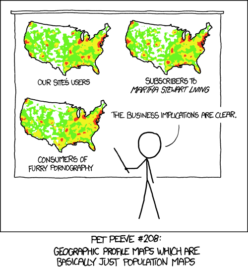
Still remember this comic from our In-Class Exercise 03? As our friends at xkcd put it, the population is not evenly distributed across the map. As such, counting-based map distributions maps roughly start representing the population instead of our topic of interest. In other words, in context of our data, townships with relatively higher total number of households will also have a higher number of households who own radios, TVs, etc. You can refer to the choropleth map comparison in section 3.2 below for an illustration of this point.
Anyways, absolute values are obviously biased towards the underlying total number of households, which isn’t what we want! 😔 Since we can’t use the absolute values, what should we do?
Never fear! We’ll derive the penetration rate of each ICT variable and use that instead:
Show code
ict_derived <- ict %>%
  mutate(`RADIO_PR` = `Radio`/`Total households`*1000) %>%
  mutate(`TV_PR` = `Television`/`Total households`*1000) %>%
  mutate(`LLPHONE_PR` = `Land line phone`/`Total households`*1000) %>%
  mutate(`MPHONE_PR` = `Mobile phone`/`Total households`*1000) %>%
  mutate(`COMPUTER_PR` = `Computer`/`Total households`*1000) %>%
  mutate(`INTERNET_PR` = `Internet at home`/`Total households`*1000) %>%
  rename(`DT_PCODE` =`District Pcode`,`DT`=`District Name`,
         `TS_PCODE`=`Township Pcode`, `TS`=`Township Name`,
         `TT_HOUSEHOLDS`=`Total households`,
         `RADIO`=`Radio`, `TV`=`Television`,
         `LLPHONE`=`Land line phone`, `MPHONE`=`Mobile phone`,
         `COMPUTER`=`Computer`, `INTERNET`=`Internet at home`)
Let’s review the summary statistics of the newly derived penetration rates:
Show code
summary(ict_derived)
   DT_PCODE              DT              TS_PCODE
 Length:55          Length:55          Length:55
 Class :character   Class :character   Class :character
 Mode  :character   Mode  :character   Mode  :character


      TS            TT_HOUSEHOLDS       RADIO             TV
 Length:55          Min.   : 3318   Min.   :  115   Min.   :  728
 Class :character   1st Qu.: 8711   1st Qu.: 1260   1st Qu.: 3744
 Mode  :character   Median :13685   Median : 2497   Median : 6117
                    Mean   :18369   Mean   : 4487   Mean   :10183
                    3rd Qu.:23471   3rd Qu.: 6192   3rd Qu.:13906
                    Max.   :82604   Max.   :30176   Max.   :62388
    LLPHONE           MPHONE         COMPUTER         INTERNET
 Min.   :  20.0   Min.   :  150   Min.   :  20.0   Min.   :   8.0
 1st Qu.: 266.5   1st Qu.: 2037   1st Qu.: 121.0   1st Qu.:  88.0
 Median : 695.0   Median : 3559   Median : 244.0   Median : 316.0
 Mean   : 929.9   Mean   : 6470   Mean   : 575.5   Mean   : 760.2
 3rd Qu.:1082.5   3rd Qu.: 7177   3rd Qu.: 507.0   3rd Qu.: 630.5
 Max.   :6736.0   Max.   :48461   Max.   :6705.0   Max.   :9746.0
    RADIO_PR          TV_PR         LLPHONE_PR       MPHONE_PR
 Min.   : 21.05   Min.   :116.0   Min.   :  2.78   Min.   : 36.42
 1st Qu.:138.95   1st Qu.:450.2   1st Qu.: 22.84   1st Qu.:190.14
 Median :210.95   Median :517.2   Median : 37.59   Median :305.27
 Mean   :215.68   Mean   :509.5   Mean   : 51.09   Mean   :314.05
 3rd Qu.:268.07   3rd Qu.:606.4   3rd Qu.: 69.72   3rd Qu.:428.43
 Max.   :484.52   Max.   :842.5   Max.   :181.49   Max.   :735.43
  COMPUTER_PR      INTERNET_PR
 Min.   : 3.278   Min.   :  1.041
 1st Qu.:11.832   1st Qu.:  8.617
 Median :18.970   Median : 22.829
 Mean   :24.393   Mean   : 30.644
 3rd Qu.:29.897   3rd Qu.: 41.281
 Max.   :92.402   Max.   :117.985
Six new fields have been added into the data.frame: RADIO_PR, TV_PR, LLPHONE_PR, MPHONE_PR, COMPUTER_PR, and INTERNET_PR.
2.5 Data Preparation
Let’s perform a relational join to update the attribute data of shan_sf (geospatial) with the attribute fields of our ict_dervied data.frame object (aspatial). We’ll do this with left_join():
Show code
#output: the data fields from ict_derived are now updated into the data frame of shan_sf
shan_sf <- left_join(shan_sf,
                     ict_derived,
                     by=c("TS_PCODE"="TS_PCODE"))
3.0 Exploratory Data Analysis (EDA)
3.1 EDA using statistical graphics
Let’s conduct EDA to find the distribution of variables. One great visualisation method is to use a histogram, which easily identifies the overall distribution/skewness of the data values (i.e. left skew, right skew or normal distribution). We’ll use RADIO:
Show code
ggplot(data=ict_derived,
       aes(x=`RADIO`)) +
  geom_histogram(bins=20,
                 color="black",
                 fill="light blue")

Meanwhile, if we’d like to detect outliers, we should look to boxplot:
Show code
ggplot(data=ict_derived,
       aes(x=`RADIO`)) +
  geom_boxplot(color="black",
               fill="light blue")

Let’s also plot the distribution of the newly derived variables. We’ll use RADIO_PR:
Show code
ggplot(data=ict_derived,
       aes(x=`RADIO_PR`)) +
  geom_histogram(bins=20,
                 color="black",
                 fill="light blue")

Show code
ggplot(data=ict_derived,
       aes(x=`RADIO_PR`)) +
  geom_boxplot(color="black",
               fill="light blue")

As we can see, the histogram for our original variable RADIO is right-skewed, with extremely far-out outliers (over six times the amount at 50th perenctile!) which means an extensive range. On the flip side, RADIO_PR has a relatively normal distribution that is slightly right-skewed, and its range is far more contained. Also notice the difference in the range of the 25th-to-50th percentile, and 50th-to-75th percentile for both: RADIO has the latter being significantly longer in range than the former, while RADIO_PR has them around the same length.
Let’s use multiple histograms to reveal the distribution of the selected variables in the ict_derived data.frame:
Show code
radio <- ggplot(data=ict_derived,
             aes(x= `RADIO_PR`)) +
  geom_histogram(bins=20,
                 color="black",
                 fill="light blue")
tv <- ggplot(data=ict_derived,
             aes(x= `TV_PR`)) +
  geom_histogram(bins=20,
                 color="black",
                 fill="light blue")
llphone <- ggplot(data=ict_derived,
             aes(x= `LLPHONE_PR`)) +
  geom_histogram(bins=20,
                 color="black",
                 fill="light blue")
mphone <- ggplot(data=ict_derived,
             aes(x= `MPHONE_PR`)) +
  geom_histogram(bins=20,
                 color="black",
                 fill="light blue")
computer <- ggplot(data=ict_derived,
             aes(x= `COMPUTER_PR`)) +
  geom_histogram(bins=20,
                 color="black",
                 fill="light blue")
internet <- ggplot(data=ict_derived,
             aes(x= `INTERNET_PR`)) +
  geom_histogram(bins=20,
                 color="black",
                 fill="light blue")
ggarrange(radio, tv, llphone, mphone, computer, internet, ncol = 3, nrow = 2)

Introducing the ggarange() function of the ggpubr package! It’s used to group the histograms together.
3.2 EDA using choropleth map
Let’s use a choropleth map to have a look at the distribution of the Radio penetration rate of Shan State (at township level):
Show code
qtm(shan_sf, "RADIO_PR")

Now, let’s compare RADIO to RADIO_PR. We’ll start by looking at the dsitribution of total number of households and number of radios:
In fact, let’s illustrate that point:
Show code
TT_HOUSEHOLDS.map <- tm_shape(shan_sf) +
  tm_fill(col = "TT_HOUSEHOLDS",
          n = 5,
          style = "jenks",
          title = "Total households") +
  tm_borders(alpha = 0.5)
RADIO.map <- tm_shape(shan_sf) +
  tm_fill(col = "RADIO",
          n = 5,
          style = "jenks",
          title = "Number Radio ") +
  tm_borders(alpha = 0.5)
tmap_arrange(TT_HOUSEHOLDS.map, RADIO.map,
             asp=NA, ncol=2)

Notice that townships with relatively larger number of households also have a relatively higher number of radio ownership. Now, let’s look at the distribution of total number of households and Radio penetration rate:
Show code

There’s a marked difference between that RADIO choropleth map and the RADIO_PR one: instead of having high densities of radio ownership in the same areas with high levels of households (mostly in the Central areas of the map), we see the more representative penetration rate (where the highest density is in the extremities of the map, one in the North, one in the West and one in the East).
3.3 Correlation Analysis
Before we perform cluster analysis, we need to perform correlation analysis so as to ensure that the cluster variables are not highly correlated. “Why?” Well - each variable gets a different weight in cluster analysis. But if you have two variables that are highly correlated (aka collinear) - the concept they represent is effectively similar, and that concept gets twice the weight as other variables since it has two contributor variables. Our solution would hence be skewed towards that concept, which is undesirable. You can read more about it on this article.

We’ll use use corrplot.mixed() function of the corrplot package to visualise and analyse the correlation of the input variables.
Show code
cluster_vars.cor = cor(ict_derived[,12:17])
corrplot.mixed(cluster_vars.cor,
         lower = "ellipse",
               upper = "number",
               tl.pos = "lt",
               diag = "l",
               tl.col = "black")

The correlation plot above shows that COMPUTER_PR and INTERNET_PR are highly correlated, which makes sense considering that a good portion of internet users access it through desktops and laptops. Knowing this, we should only use one of them in the cluster analysis instead of both.
4.0 Hierarchy Cluster Analysis
4.1 Extrating clustering variables
Firstly, we’ll extract the clustering variables from the shan_sf:
Show code
cluster_vars <- shan_sf %>%
  st_set_geometry(NULL) %>%
  select("TS.x", "RADIO_PR", "TV_PR", "LLPHONE_PR", "MPHONE_PR", "COMPUTER_PR")
head(cluster_vars,10)
        TS.x RADIO_PR    TV_PR LLPHONE_PR MPHONE_PR COMPUTER_PR
1    Mongmit 286.1852 554.1313   35.30618  260.6944    12.15939
2    Pindaya 417.4647 505.1300   19.83584  162.3917    12.88190
3    Ywangan 484.5215 260.5734   11.93591  120.2856     4.41465
4   Pinlaung 231.6499 541.7189   28.54454  249.4903    13.76255
5     Mabein 449.4903 708.6423   72.75255  392.6089    16.45042
6      Kalaw 280.7624 611.6204   42.06478  408.7951    29.63160
7      Pekon 318.6118 535.8494   39.83270  214.8476    18.97032
8   Lawksawk 387.1017 630.0035   31.51366  320.5686    21.76677
9  Nawnghkio 349.3359 547.9456   38.44960  323.0201    15.76465
10   Kyaukme 210.9548 601.1773   39.58267  372.4930    30.94709
Note that the final clustering variables list does not include variable INTERNET_PR - as we’ve found from our 3.3 Correlation Analysis, it’s highly correlated with the variable COMPUTER_PR, so we’re using the latter only.
Next, we need to change the rows by township name instead of row number:
               TS.x RADIO_PR    TV_PR LLPHONE_PR MPHONE_PR
Mongmit     Mongmit 286.1852 554.1313   35.30618  260.6944
Pindaya     Pindaya 417.4647 505.1300   19.83584  162.3917
Ywangan     Ywangan 484.5215 260.5734   11.93591  120.2856
Pinlaung   Pinlaung 231.6499 541.7189   28.54454  249.4903
Mabein       Mabein 449.4903 708.6423   72.75255  392.6089
Kalaw         Kalaw 280.7624 611.6204   42.06478  408.7951
Pekon         Pekon 318.6118 535.8494   39.83270  214.8476
Lawksawk   Lawksawk 387.1017 630.0035   31.51366  320.5686
Nawnghkio Nawnghkio 349.3359 547.9456   38.44960  323.0201
Kyaukme     Kyaukme 210.9548 601.1773   39.58267  372.4930
          COMPUTER_PR
Mongmit      12.15939
Pindaya      12.88190
Ywangan       4.41465
Pinlaung     13.76255
Mabein       16.45042
Kalaw        29.63160
Pekon        18.97032
Lawksawk     21.76677
Nawnghkio    15.76465
Kyaukme      30.94709
Success! The row number has been replaced into the township name.
From there, let’s delete the TS.x field:
          RADIO_PR    TV_PR LLPHONE_PR MPHONE_PR COMPUTER_PR
Mongmit   286.1852 554.1313   35.30618  260.6944    12.15939
Pindaya   417.4647 505.1300   19.83584  162.3917    12.88190
Ywangan   484.5215 260.5734   11.93591  120.2856     4.41465
Pinlaung  231.6499 541.7189   28.54454  249.4903    13.76255
Mabein    449.4903 708.6423   72.75255  392.6089    16.45042
Kalaw     280.7624 611.6204   42.06478  408.7951    29.63160
Pekon     318.6118 535.8494   39.83270  214.8476    18.97032
Lawksawk  387.1017 630.0035   31.51366  320.5686    21.76677
Nawnghkio 349.3359 547.9456   38.44960  323.0201    15.76465
Kyaukme   210.9548 601.1773   39.58267  372.4930    30.94709
4.2 Data Standardisation
When multiple variables are used, we’d normally see a difference in the range of their values. However, our analysis will tend to be biased to variables with larger values. To illustrate this point…
Imagine that we’re trying to determine a person’s level of wealth, and we have the variables “money in their wallet” and “number of houses they own”.

Person A has $100 in their wallet, owns 5 houses. Person B has $10,000 in their wallet, owns 1 house.
As humans, our first thought might be “how does Person A afford 5 houses!?” - we know that having more houses is a better indicator wealth than cash. But our analysis only looks at the difference - “a difference of 9,900 is more significant than a difference of 4” - and then assign a greater weight to “money in their wallet”.
As such, to prevent such a case from happening, we’ll need to standardise the input variables.
4.2.1 Min-Max standardisation
We’ll use normalize() of the heatmaply package to standardise using the Min-Max method, and display the summary statistics with summary().
Show code
shan_ict.std <- normalize(shan_ict)
summary(shan_ict.std)
    RADIO_PR          TV_PR          LLPHONE_PR       MPHONE_PR
 Min.   :0.0000   Min.   :0.0000   Min.   :0.0000   Min.   :0.0000
 1st Qu.:0.2544   1st Qu.:0.4600   1st Qu.:0.1123   1st Qu.:0.2199
 Median :0.4097   Median :0.5523   Median :0.1948   Median :0.3846
 Mean   :0.4199   Mean   :0.5416   Mean   :0.2703   Mean   :0.3972
 3rd Qu.:0.5330   3rd Qu.:0.6750   3rd Qu.:0.3746   3rd Qu.:0.5608
 Max.   :1.0000   Max.   :1.0000   Max.   :1.0000   Max.   :1.0000
  COMPUTER_PR
 Min.   :0.00000
 1st Qu.:0.09598
 Median :0.17607
 Mean   :0.23692
 3rd Qu.:0.29868
 Max.   :1.00000
Note that the values range of the Min-max standardised clustering variables are 0-1 now.
4.2.2 Z-score standardisation
For Z-score standardisation, we assume all variables come from some normal distribution. If we know otherwise, it should not be used. We’ll use scale() of Base R to perform Z-score standardisation. We’ll also use describe() of psych package instead of summary() since it provides the standard deviation.
Show code
shan_ict.z <- scale(shan_ict)
describe(shan_ict.z)
            vars  n mean sd median trimmed  mad   min  max range
RADIO_PR       1 55    0  1  -0.04   -0.06 0.94 -1.85 2.55  4.40
TV_PR          2 55    0  1   0.05    0.04 0.78 -2.47 2.09  4.56
LLPHONE_PR     3 55    0  1  -0.33   -0.15 0.68 -1.19 3.20  4.39
MPHONE_PR      4 55    0  1  -0.05   -0.06 1.01 -1.58 2.40  3.98
COMPUTER_PR    5 55    0  1  -0.26   -0.18 0.64 -1.03 3.31  4.34
             skew kurtosis   se
RADIO_PR     0.48    -0.27 0.13
TV_PR       -0.38    -0.23 0.13
LLPHONE_PR   1.37     1.49 0.13
MPHONE_PR    0.48    -0.34 0.13
COMPUTER_PR  1.80     2.96 0.13
Note that the mean and standard deviation of the Z-score standardised clustering variables are 0 and 1 respectively.
4.2.3 Visualising the standardised clustering variables
Other than reviewing the summary statistics of the standardised clustering variables, let’s visualise their distribution graphical as well!
Show code
r <- ggplot(data=ict_derived,
             aes(x= `RADIO_PR`)) +
  geom_histogram(bins=20,
                 color="black",
                 fill="light blue")
shan_ict_s_df <- as.data.frame(shan_ict.std)
s <- ggplot(data=shan_ict_s_df,
       aes(x=`RADIO_PR`)) +
  geom_histogram(bins=20,
                 color="black",
                 fill="light blue") +
  ggtitle("Min-Max Standardisation")
shan_ict_z_df <- as.data.frame(shan_ict.z)
z <- ggplot(data=shan_ict_z_df,
       aes(x=`RADIO_PR`)) +
  geom_histogram(bins=20,
                 color="black",
                 fill="light blue") +
  ggtitle("Z-score Standardisation")
ggarrange(r, s, z,
          ncol = 3,
          nrow = 1)

Did you notice? 💡 The overall distribution of the clustering variables will change after the data standardisation. However, take note that we should NOT perform data standardisation if the values range of the clustering variables isn’t very large.
4.3 Computing proximity matrix
Let’s compute the proximity matrix by using dist() of R. dist() supports six distance proximity calculations:
- euclidean
- maximum
- manhattan
- canberra
- binary
- minkowski
The default is euclidean proximity matrix.
Here, we’ll compute the proximity matrix using euclidean method:
Show code
proxmat <- dist(shan_ict, method = 'euclidean')
Let’s inspect the content of proxmat:
Show code
proxmat
4.4 Computing hierarchical clustering
While there are several packages which provide hierarchical clustering functions, in this exercise, we’ll be introducing the hclust() function of R stats. It employs the agglomeration method to compute the cluster, and supports 8 clustering algorithms: ward.D, ward.D2, single, complete, average(UPGMA), mcquitty(WPGMA), median(WPGMC) and centroid(UPGMC).
We’ll try the ward.D method for our hierarchcial cluster analysis:
Show code
# output: hclust class object which describes the tree produced by the clustering process
hclust_ward <- hclust(proxmat, method = 'ward.D')
We can then plot() the tree:
Show code
plot(hclust_ward, cex = 0.6)

4.5 Selecting the optimal clustering algorithm
One of the main challenges of hierarchical clustering is how to identify stronger clustering structures. To address this, we use the agnes() function of the cluster package. It functions like hclust but with the added benefit of the agglomerative coefficient, which measures the amount of clustering structure found, with Values closer to 1 suggesting a strong clustering structure.
Let’s compute the agglomerative coefficients of all hierarchical clustering algorithms to see which ones has the strongest clsutering structure!
Show code
  average    single  complete      ward
0.8131144 0.6628705 0.8950702 0.9427730
DING-DING-DING! We have a winner: Ward’s method provides the strongest clustering structure among the four methods assessed. Hence, only Ward’s method will be used in the subsequent analysis.
4.6 Determining Optimal Clusters
Another technical challenge faced when performing clustering analysis is how to determine the optimal clusters to retain. There are three commonly used methods to determine the optimal clusters:
For this exercise, we’ll be using the gap statistic method.
Gap Statistic Method
The gap statistic compares the total within intra-cluster variation for different values of k with their expected values under null reference distribution of the data. The estimate of the optimal clusters will be the value that maximizes the gap statistic. This also implies that the clustering structure is far away from the random uniform distribution of points.
To compute the gap statistic, we’ll use the clusGap() function of the cluster package. We’ll also be using the the hcut function from the factoextra package.
Show code
Clustering Gap statistic ["clusGap"] from call:
clusGap(x = shan_ict, FUNcluster = hcut, K.max = 10, B = 50,     nstart = 25)
B=50 simulated reference sets, k = 1..10; spaceH0="scaledPCA"
 --> Number of clusters (method 'firstmax'): 1
          logW   E.logW       gap     SE.sim
 [1,] 8.407129 8.680794 0.2736651 0.04460994
 [2,] 8.130029 8.350712 0.2206824 0.03880130
 [3,] 7.992265 8.202550 0.2102844 0.03362652
 [4,] 7.862224 8.080655 0.2184311 0.03784781
 [5,] 7.756461 7.978022 0.2215615 0.03897071
 [6,] 7.665594 7.887777 0.2221833 0.03973087
 [7,] 7.590919 7.806333 0.2154145 0.04054939
 [8,] 7.526680 7.731619 0.2049390 0.04198644
 [9,] 7.458024 7.660795 0.2027705 0.04421874
[10,] 7.377412 7.593858 0.2164465 0.04540947
Next, we’ll visualise the plot by using the fviz_gap_stat() function of factoextra package:
Show code
fviz_gap_stat(gap_stat)

Hmm… as we can see, the recommended number of clusters to retain is 1. But that simply isn’t logical - one cluster would mean that the whole map is one big cluster, which defeats the purpose of cluster analysis and segmentation 😟
Looking at the gap statistic graph, the 6-cluster gives the largest gap statistic - so we’ll pick that as our best choice.
4.7 Interpreting the dendrograms
What is a dendrogram? In a dendrogram, each leaf corresponds to one observation. As we move up the tree, observations that are similar to each other are combined into branches, which are themselves fused at a higher height.
The height of the fusion, provided on the vertical axis, indicates the (dis)similarity between two observations. The higher the height of the fusion, the less similar the observations are. Take note that conclusions about the proximity of two observations can be drawn only based on the height where branches containing those two observations first are fused. We cannot use the proximity of two observations along the horizontal axis as a criteria of their similarity.
Let’s try plotting a dendrogram with a border around the selected clusters by using the rect.hclust() function of R stats:
Show code
plot(hclust_ward, cex = 0.6)
rect.hclust(hclust_ward,
            k = 6,
            # specify border colours for rectangles
            border = 2:5)

4.8 Visually-driven hierarchical clustering analysis
In this section, we’ll be building highly interactive or static cluster heatmaps with the heatmaply package.
4.8.1 Transforming the data frame into a matrix
For heatmaps, our data has to be in a data matrix:
Show code
shan_ict_mat <- data.matrix(shan_ict)
4.8.2 Plotting interactive cluster heatmap using heatmaply()
Now, we’ll use the heatmaply() function of the heatmaply package to build an interactive cluster heatmap:
Show code
heatmaply(normalize(shan_ict_mat),
          Colv=NA,
          dist_method = "euclidean",
          hclust_method = "ward.D",
          seriate = "OLO",
          colors = Blues,
          k_row = 6,
          margins = c(NA,200,60,NA),
          fontsize_row = 4,
          fontsize_col = 5,
          main="Geographic Segmentation of Shan State by ICT indicators",
          xlab = "ICT Indicators",
          ylab = "Townships of Shan State"
          )
4.9 Mapping the clusters formed
Using the cutree() function of Base R, we’ll derive 6-cluster model.
Since our output is a list object, we’ll need to append it back on shan_sf to visualise our clusters. Firstly, we’ll convert groups into a matrix, then append it onto shan_sf with cbind(), and while we’re at it - we’ll rename the as.matrix.groups field as CLUSTER.
Next, let’s have a quick plot of a choropleth map of the clusters formed:
Show code
qtm(shan_sf_cluster, "CLUSTER")

As we can see from our choropleth map above, the clusters are very fragmented. The tends to be one of the major limitations when non-spatial clustering algorithm (in this case, hierarchical clustering) is used.
5.0 Spatially Constrained Clustering - SKATER approach
Well, now that we know what a non-spatial clustering algorithm is like, what about spatial clustering algorithms? In this section, we’ll learn how derive spatially constrained cluster by using the skater() method of the spdep package.
5.1 Converting into SpatialPolygonsDataFrame
While our heatmaps needed a matrix format, our SKATER function only supports sp objects. As such, we’ll need to convert shan_sf into SpatialPolygonsDataFrame with the as_Spatial() method:
Show code
shan_sp <- as_Spatial(shan_sf)
5.2 Computing Neighbour List
Next, we’ll use poly2nd() to compute the neighbours list from polygon list:
Show code
shan.nb <- poly2nb(shan_sp)
summary(shan.nb)
Neighbour list object:
Number of regions: 55
Number of nonzero links: 264
Percentage nonzero weights: 8.727273
Average number of links: 4.8
Link number distribution:

 2  3  4  5  6  7  8  9
 5  9  7 21  4  3  5  1
5 least connected regions:
3 5 7 9 47 with 2 links
1 most connected region:
8 with 9 links
Now, let’s get to plotting. Since we can now plot the community area boundaries as well,let’s plot that graph on top of the map, like so:
Show code

NOTE: if you plot the network first and then the boundaries, some of the areas will be clipped. This is because the plotting area is determined by the characteristics of the first plot. In this example, since the boundary map extends further than the graph, we should plot it first.
5.3 Computing minimum spanning tree
5.3.1 Calculating edge costs
We’ll use nbcosts() of the spdep package to compute the cost of each edge aka the distance between nodes:
Show code
lcosts <- nbcosts(shan.nb, shan_ict)
This is the notion of a generalised weight for a spatial weights matrix: for each observation, this gives the pairwise dissimilarity between its values on the five variables and the values for the neighbouring observation (from the neighbour list).
Next, let’s incorporate these costs into a weights object the same way we did in the calculation of inverse of distance weights: we’ll convert it into a list weights object by specifying the just computed lcosts as the weights. We’ll use nb2listw(), like so:.
Show code
# style="B" to make sure that the cost values are not row-standardised
shan.w <- nb2listw(shan.nb,
                   lcosts,
                   style="B")
summary(shan.w)
Characteristics of weights list object:
Neighbour list object:
Number of regions: 55
Number of nonzero links: 264
Percentage nonzero weights: 8.727273
Average number of links: 4.8
Link number distribution:

 2  3  4  5  6  7  8  9
 5  9  7 21  4  3  5  1
5 least connected regions:
3 5 7 9 47 with 2 links
1 most connected region:
8 with 9 links

Weights style: B
Weights constants summary:
   n   nn       S0       S1        S2
B 55 3025 76267.65 58260785 522016004
5.3.2 Computing minimum spanning tree
We’ll compute the minimum spanning tree with mstree():
Show code
shan.mst <- mstree(shan.w)
After computing the MST, we can check its class and dimension:
“Wait a moment, why is the dimension 54 and not 55?” You might be wondering. Don’t worry: this happens because the minimum spanning tree consists on n-1 edges (links) in order to traverse all the nodes.
Let’s also display the content of shan.mst:
Show code
head(shan.mst)
     [,1] [,2]      [,3]
[1,]   31   25 229.44658
[2,]   25   10 163.95741
[3,]   10    1 144.02475
[4,]   10    9 157.04230
[5,]    9    8  90.82891
[6,]    8    6 140.01101
Now that we have a rough overview of our MST, it’s time to plot! Our goal is to see how the initial neighbour list is simplified to just one edge connecting each of the nodes, while passing through all the nodes. Like before, we’ll plot it together with the township boundaries.
Show code

5.4 Computing spatially constrained clusters using SKATER method
Now to the meat of the section! Let’s compute the spatially constrained cluster using skater():
Show code
clust6 <- skater(edges = shan.mst[,1:2],
                 data = shan_ict,
                 method = "euclidean",
                 ncuts = 5)
The skater() method takes three mandatory arguments: - the first two columns of the MST matrix (i.e. not the cost) - the data matrix (to update the costs as units are being grouped) - the number of cuts. Note that it is set to one less than the number of clusters to represent the number of cuts
Show code
str(clust6)
List of 8
 $ groups      : num [1:55] 3 3 6 3 3 3 3 3 3 3 ...
 $ edges.groups:List of 6
  ..$ :List of 3
  .. ..$ node: num [1:22] 13 48 54 55 45 37 34 16 25 31 ...
  .. ..$ edge: num [1:21, 1:3] 48 55 54 37 34 16 45 31 13 13 ...
  .. ..$ ssw : num 3423
  ..$ :List of 3
  .. ..$ node: num [1:18] 47 27 53 38 42 15 41 51 43 32 ...
  .. ..$ edge: num [1:17, 1:3] 53 15 42 38 41 51 15 27 15 43 ...
  .. ..$ ssw : num 3759
  ..$ :List of 3
  .. ..$ node: num [1:11] 2 6 8 1 36 4 10 9 46 5 ...
  .. ..$ edge: num [1:10, 1:3] 6 1 8 36 4 6 8 10 10 9 ...
  .. ..$ ssw : num 1458
  ..$ :List of 3
  .. ..$ node: num [1:2] 44 20
  .. ..$ edge: num [1, 1:3] 44 20 95
  .. ..$ ssw : num 95
  ..$ :List of 3
  .. ..$ node: num 23
  .. ..$ edge: num[0 , 1:3]
  .. ..$ ssw : num 0
  ..$ :List of 3
  .. ..$ node: num 3
  .. ..$ edge: num[0 , 1:3]
  .. ..$ ssw : num 0
 $ not.prune   : NULL
 $ candidates  : int [1:6] 1 2 3 4 5 6
 $ ssto        : num 12613
 $ ssw         : num [1:6] 12613 10977 9962 9540 9123 ...
 $ crit        : num [1:2] 1 Inf
 $ vec.crit    : num [1:55] 1 1 1 1 1 1 1 1 1 1 ...
 - attr(*, "class")= chr "skater"
Did you notice? The grouops vector contains labels of hte cluster to which each observation belongs - followed by a detailed summary for each of the clustesr in edges.groups. Also take note that the sum of squares measures are given as ssto for the total and ssw to show the effect of each of the cuts on the overall criterion.
Let’s check the cluster assignment:
Show code
ccs6 <- clust6$groups
ccs6
 [1] 3 3 6 3 3 3 3 3 3 3 2 1 1 1 2 1 1 1 2 4 1 2 5 1 1 1 2 1 2 2 1 2 2
[34] 1 1 3 1 2 2 2 2 2 2 4 1 3 2 1 1 1 2 1 2 1 1
We can also check the number of observations per cluster with table():
Show code
table(ccs6)
ccs6
 1  2  3  4  5  6
22 18 11  2  1  1
Lastly, let’s plot the pruned tree that shows the five clusters on top of the townshop area:
Show code

5.5 Visualising the clusters in choropleth map
Let’s plot the newly derived clusters by using SKATER method!
Show code

We should also compare the hierarchical clustering and spatially constrained hierarchical clustering maps:
Show code
hclust.map <- qtm(shan_sf_cluster,
                  "CLUSTER") +
  tm_borders(alpha = 0.5)
shclust.map <- qtm(shan_sf_spatialcluster,
                   "SP_CLUSTER") +
  tm_borders(alpha = 0.5)
tmap_arrange(hclust.map, shclust.map,
             asp=NA, ncol=2)

6.0 End Notes
With that, we’ve learned how to perform both non-spatial clustering and spatially-constrained clustering, from data prep to visualisation! Tune in next week for more geospatial analytics tips 😄